Habitat Data Sources • spacemodR

Introduction

A habitat layer tells, for each pixel of the landscape, how good the place is for a species and how hard it is to cross. In spacemodR it is always built the same way:

a land cover map, which splits the landscape into classes;
a species dictionary, which gives the scores of a species for each class;
a join of the two, then a rasterization on the grid shared with the other layers (soil contamination, for instance).

The Habitat Layer guide follows these steps with one map and explains how to turn the result into a habitat object. This guide is about step 1: which map to use, what each one can and cannot tell apart, and how to move from one to another.

Source	Extent	Resolution	Classes	Dictionary	Get the data
OCS-GE, cover (`CS`)	France	vector, about 1:5,000	14	`ocsge_species_dict`, rows with `code_us = NA`	`get_ocsge()`
OCS-GE, cover and use (`CS` x `US`)	France	vector, about 1:5,000	14 covers, refined for 47 (cover, use) pairs	`ocsge_species_dict`, rows with a `code_us`	`get_ocsge()`
EUNIS Level 2	39 EEA countries	raster, 100 m	45	`eunis_species_dict`	`get_eunis_data()`

The table ref_ocsge_eunis links the OCS-GE and EUNIS nomenclatures. Other sources that would refine these maps (agricultural parcels, vegetation indices, LiDAR) are discussed at the end.

All examples use the Metaleurop site, and mostly two small mammals with opposite needs: the common vole (Microtus arvalis), a species of open farmland, and the bank vole (Myodes glareolus), a species of woodland and dense cover.

library(spacemodR)
library(sf)
library(dplyr)
library(ggplot2)
library(terra)
library(tidyterra)
library(patchwork)

Species dictionaries

One schema for every source

ocsge_species_dict and eunis_species_dict cover the same 935 European terrestrial vertebrates and have the same columns. Only the column holding the land cover class differs.

data("ocsge_species_dict")
data("eunis_species_dict")
names(ocsge_species_dict)
#>  [1] "code_cs"         "code_us"         "species_name"    "sppID"          
#>  [5] "taxon_group"     "suitability"     "weight_breeding" "weight_foraging"
#>  [9] "permeability"    "resistance"      "habitat_breadth" "specialization" 
#> [13] "confidence"      "in_france"
names(eunis_species_dict)
#>  [1] "code_eunis"      "species_name"    "sppID"           "taxon_group"    
#>  [5] "suitability"     "weight_breeding" "weight_foraging" "permeability"   
#>  [9] "resistance"      "habitat_breadth" "specialization"  "confidence"     
#> [13] "in_france"

Column	Level	Range	Meaning
`code_cs`, `code_us`	class	–	OCS-GE cover and use. `code_us` is `NA` on the rows that score a cover whatever its use.
`code_eunis`	class	–	EUNIS Level 2 code, as in `ref_eunis` and in the raster returned by `get_eunis_data(level = "L2")`.
`species_name`	species	–	Scientific name, `Genus_species`.
`sppID`	species	–	EEA identifier; first letter gives the group (A, R, B, M).
`taxon_group`	species	–	amphibian, reptile, bird or mammal.
`suitability`	class	0–10	Overall habitat quality. Use as the source / habitat weight.
`weight_breeding`	class	0–10	Value as breeding, nesting, denning, roosting or larval site.
`weight_foraging`	class	0–10	Value for feeding.
`permeability`	class	0–10	Ease of movement (10 free, 7 readily, 4 reluctantly, 1 strong barrier, 0 impassable).
`resistance`	class	1–100	`10^(2 * (1 - permeability / 10))`: 10 → 1, 5 → 10, 0 → 100. Use as the resistance layer.
`habitat_breadth`	species	–	Number of classes with `suitability >= 5` (out of 14 covers or 45 EUNIS classes).
`specialization`	species	0–1	1 − normalised Shannon evenness of the suitability profile: 0 generalist, 1 specialist.
`confidence`	species	1–3	Quality of the source description: 1 vague or empty, 2 medium, 3 detailed.
`in_france`	species	0/1	1 if the species occurs natively and regularly in metropolitan France.

How the scores were built

The input is the habitat and avoided-habitat description of each species published by the EEA (O’Connor et al. 2024). A large language model (Claude Opus) read each description against a short ecological summary of every class and scored it with the same rules for all sources:

Anchored scale. Every score uses the same reference points (0 unused or avoided, 2 marginal, 5 secondary, 8 main, 10 core habitat), so that a 5 means the same thing for a toad and for an eagle.
Breeding separated from foraging. Many species breed in one habitat and feed in another (amphibians in ponds and woods, raptors on cliffs and in steppe).
Taxon-aware movement. Flight, swimming and burrowing are taken into account, so a road is a strong barrier for a toad but not for a kite.
Resistance derived, not scored. Resistance is computed from permeability on the 1–100 log scale expected by Omniscape, so the two can never contradict each other and no further transformation is needed.

data.frame(permeability = 0:10) %>%
  mutate(resistance = 10^(2 * (1 - permeability / 10))) %>%
  ggplot(aes(permeability, resistance)) +
  geom_line(colour = "#2a78d6", linewidth = 1) +
  geom_point(colour = "#2a78d6", size = 2) +
  scale_y_log10(breaks = c(1, 2.5, 10, 25, 100)) +
  scale_x_continuous(breaks = 0:10) +
  theme_minimal() +
  labs(x = "Permeability (0–10)", y = "Resistance (log scale)")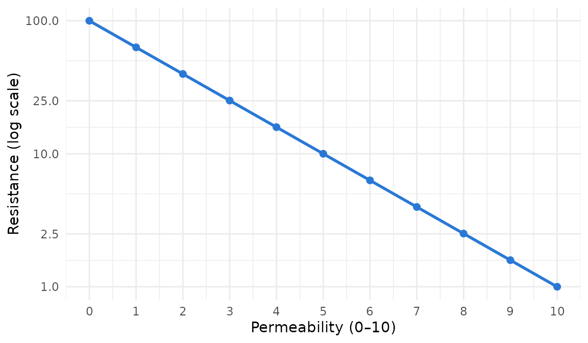

These are expert-judgement values, not values fitted to occurrence data.

Selecting species

The dictionaries cover Europe. Before working on a French site, keep the species that occur in France, and check how much is known about them:

ocsge_species_dict %>%
  distinct(species_name, taxon_group, habitat_breadth, specialization, confidence, in_france) %>%
  filter(in_france == 1, confidence == 3) %>%
  arrange(desc(specialization)) %>%
  head(8)
#>           species_name taxon_group habitat_breadth specialization confidence
#> 1           Uria_aalge        bird               0              1          3
#> 2        Gavia_arctica        bird               1              1          3
#> 3          Gavia_immer        bird               1              1          3
#> 4       Gavia_stellata        bird               1              1          3
#> 5     Podiceps_auritus        bird               1              1          3
#> 6   Podiceps_cristatus        bird               1              1          3
#> 7   Podiceps_grisegena        bird               1              1          3
#> 8 Podiceps_nigricollis        bird               1              1          3
#>   in_france
#> 1         1
#> 2         1
#> 3         1
#> 4         1
#> 5         1
#> 6         1
#> 7         1
#> 8         1

Source 1: OCS-GE land cover (CS)

OCS-GE is the French large-scale land cover database. Its couverture du sol (CS) describes what physically covers the ground, in 14 classes.

data("ocsge_metaleurop")
data("ref_ocsge")
ref_ocsge[, c("code_cs", "nomenclature")]
#>      code_cs                            nomenclature
#> 1  CS1.1.1.1                            Zones bâties
#> 2  CS1.1.1.2                        Zones non bâties
#> 3  CS1.1.2.1                      Matériaux minéraux
#> 4  CS1.1.2.2                    Matériaux composites
#> 5    CS1.2.1                                Sols nus
#> 6    CS1.2.2                          Surfaces d'eau
#> 7    CS1.2.3                       Névés et glaciers
#> 8  CS2.1.1.1                                Feuillus
#> 9  CS2.1.1.2                               Conifères
#> 10 CS2.1.1.3                                   Mixte
#> 11   CS2.1.2 Formations arbustives, sous-arbrisseaux
#> 12   CS2.1.3             Autres formations ligneuses
#> 13   CS2.2.1                    Formations herbacées
#> 14   CS2.2.2         Autres formations non ligneuses

The examples below use the layers shipped with the package. For another site, get_ocsge() returns the polygons of a region of interest, with their CS and US codes. It reads them either from the download service of IGN, which publishes one GeoPackage per department and vintage, or from a FlatGeobuf file that you host.

# IGN: the departments of the ROI are downloaded once, then read from a cache
ocsge_site <- get_ocsge(roi_metaleurop, source = "ign", year = 2021)

# FlatGeobuf: only the features of the ROI are downloaded
ocsge_site <- get_ocsge(roi_metaleurop, source = "fgb",
                        fgb_url = "https://example.com/data/ocsge_france.fgb")

join_ocsge_species() adds the scores of a species to the polygons, and plot_species_habitat() maps them.

microtus_cs <- join_ocsge_species(ocsge_metaleurop, "Microtus_arvalis")
plot_species_habitat(microtus_cs)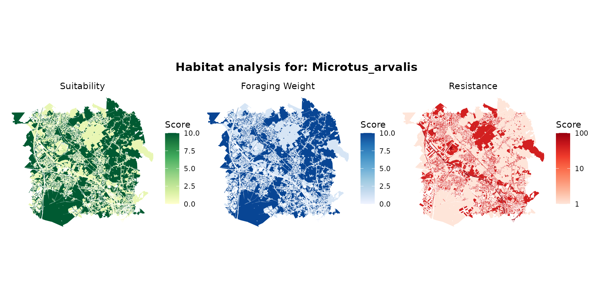

The strength of this source is its geometry: buildings, roads, hedges and ponds a few meters wide are mapped. Its weakness is that 14 cover classes say little about habitats. Herbaceous cover (CS2.2.1) holds cereal fields, meadows, lawns, road verges and reedbeds alike, and a species gets a single score for all of them:

ocsge_species_dict %>%
  filter(code_cs == "CS2.2.1", is.na(code_us),
         species_name %in% c("Microtus_arvalis", "Myodes_glareolus")) %>%
  select(species_name, code_cs, suitability, weight_foraging, permeability)
#>       species_name code_cs suitability weight_foraging permeability
#> 1 Microtus_arvalis CS2.2.1          10              10           10
#> 2 Myodes_glareolus CS2.2.1           3               3            5

Source 2: OCS-GE land cover and land use (CS x US)

What the use adds

OCS-GE polygons also carry an usage du sol (US): agriculture, forestry, residential, transport networks, and so on. The use does not describe a habitat by itself, but it tells what a cover stands for. On the Metaleurop site, herbaceous cover is made of:

data("ocsge_us_metaleurop")
ocsge_us_metaleurop %>%
  st_drop_geometry() %>%
  filter(code_cs == "CS2.2.1") %>%
  arrange(desc(area_ha)) %>%
  mutate(share = round(100 * area_ha / sum(area_ha)))
#>    code_cs code_us area_ha share
#> 1  CS2.2.1   US1.1 1581.64    62
#> 2  CS2.2.1     US5  523.07    21
#> 3  CS2.2.1     US3  188.80     7
#> 4  CS2.2.1   US6.3  110.41     4
#> 5  CS2.2.1 US4.1.1   48.81     2
#> 6  CS2.2.1     US2   44.53     2
#> 7  CS2.2.1   US4.2   30.03     1
#> 8  CS2.2.1   US1.3    9.76     0
#> 9  CS2.2.1   US4.3    8.56     0
#> 10 CS2.2.1 US4.1.2    2.13     0
#> 11 CS2.2.1   US6.1    0.27     0

Crops (US1.1, agriculture) make more than half of it, and gardens (US5, residential) about a fifth. ocsge_species_dict has rows for the (cover, use) pairs where the use matters:

ocsge_species_dict %>%
  filter(code_cs == "CS2.2.1",
         species_name %in% c("Microtus_arvalis", "Myodes_glareolus"),
         is.na(code_us) | code_us %in% c("US1.1", "US1.2", "US3", "US5", "US6.3")) %>%
  select(species_name, code_us, suitability) %>%
  tidyr::pivot_wider(names_from = species_name, values_from = suitability)
#> # A tibble: 6 × 3
#>   code_us Microtus_arvalis Myodes_glareolus
#>   <chr>              <int>            <int>
#> 1 NA                    10                3
#> 2 US1.1                  9                1
#> 3 US1.2                  5                6
#> 4 US3                    7                4
#> 5 US5                    7                4
#> 6 US6.3                  8                1

For the bank vole, herbaceous cover is poor habitat as a whole, almost unused when it is farmed, and secondary habitat when it is a forest clearing (US1.2). The common vole shows the opposite pattern.

Rows with a code_us are not scored one by one: each (cover, use) pair is linked to EUNIS classes by ref_ocsge_eunis (see below) and takes a weighted mean of their scores in eunis_species_dict.

Joining on cover and use

When the spatial object has a code_us column, join_ocsge_species() uses it. A polygon takes the scores of its (cover, use) pair when the dictionary has one, and the scores of its cover otherwise; the column use_matched tells which.

myodes_us <- join_ocsge_species(ocsge_us_metaleurop, "Myodes_glareolus")

myodes_us %>%
  st_drop_geometry() %>%
  group_by(use_matched) %>%
  summarise(pairs = n(), area_ha = round(sum(area_ha)))
#> # A tibble: 2 × 3
#>   use_matched pairs area_ha
#>   <lgl>       <int>   <dbl>
#> 1 FALSE          40    1961
#> 2 TRUE           28    2841

To ignore the use, set us_col = NULL. The maps below compare the two for the bank vole:

myodes_cs <- join_ocsge_species(ocsge_us_metaleurop, "Myodes_glareolus", us_col = NULL)

map_suit <- function(x, title) {
  ggplot(x) +
    geom_sf(aes(fill = suitability), color = NA) +
    scale_fill_gradient(low = "#ffffe5", high = "#004529", limits = c(0, 10),
                        na.value = "transparent", name = "Suitability") +
    theme_void() +
    labs(title = title)
}
map_suit(myodes_cs, "Cover only") + map_suit(myodes_us, "Cover and use") +
  plot_layout(guides = "collect") +
  plot_annotation(title = "Myodes glareolus")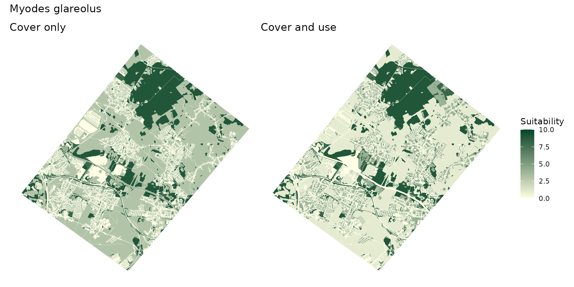

With the cover alone, every field and garden is poor habitat of the same value. With the use, farmland drops to almost nothing, while gardens, parks and forest clearings keep some value.

What the use cannot tell

Some distinctions remain out of reach of OCS-GE, with or without the use:

crops and permanent grassland share the same cover and the same agricultural use;
wetlands (reedbeds, wet meadows, bogs) are not identified;
grassland types (dry, mesic, wet, alpine) are not separated;
standing and running water, deciduous and evergreen broadleaved woodland are not separated.

Source 3: EUNIS

When to use it

EUNIS (European Nature Information System) is a habitat classification. The EEA Ecosystem Type Map v3.1 maps it over the 39 EEA countries at 100 m. It is the source to use when:

the study area is outside France;
the species depends on habitats that OCS-GE cannot separate. EUNIS Level 2 has 45 terrestrial classes, including 6 wetland types (D1–D6), 6 grassland types (E1–E7) and 10 scrub types (F1–FB).

The trade-off is resolution: one pixel of 100 m carries a single dominant class, so roads, hedges and gardens disappear into their surroundings.

The EUNIS land cover layer

get_eunis_data() downloads the EUNIS raster for any region of interest from the EEA map service. To keep this guide reproducible offline, the Metaleurop layer is kept in the source repository (inst/extdata/eunis_metaleurop_L2.tif, read here with a small helper, load_raster_repo()); it was produced with:

data("roi_metaleurop")
eunis_lc <- get_eunis_data(roi_metaleurop, level = "L2", resolution = 100)

data("ref_eunis")
ref_l2 <- ref_eunis %>% filter(level == "L2") %>% select(code, nomenclature, couleur)

eunis_lc <- load_raster_repo("eunis_metaleurop_L2.tif")
lv <- terra::levels(eunis_lc)[[1]]
names(lv) <- c("value", "code")
lv %>% left_join(ref_l2, by = "code") %>% select(code, nomenclature)
#>     code                                                 nomenclature
#> 1     C1                                      Surface standing waters
#> 2  D5/F6                                                         <NA>
#> 3     E2                                             Mesic grasslands
#> 4     F4                                    Temperate shrub heathland
#> 5     G1                               Broadleaved deciduous woodland
#> 6     G3                                          Coniferous woodland
#> 7     G4                      Mixed deciduous and coniferous woodland
#> 8     I1                               Arable land and market gardens
#> 9     I2                        Cultivated areas of gardens and parks
#> 10    J1                      Buildings of cities, towns and villages
#> 11    J2                                        Low density buildings
#> 12    J3                                  Extractive industrial sites
#> 13    J4 Transport networks and other constructed hard-surfaced areas
#> 14    J6                                               Waste deposits

The raster is categorical. Note the combined code "D5/F6": the EEA service draws D5 (sedge and reedbeds) and F6 (garrigue) with the same color, so these pixels cannot be told apart (see ?get_eunis_data).

eunis_lab <- lv %>%
  left_join(ref_l2, by = "code") %>%
  transmute(value,
            eunis = ifelse(is.na(nomenclature), code, paste(code, substr(nomenclature, 1, 40))),
            couleur = ifelse(is.na(couleur), "#BDBDBD", couleur))
eunis_lc_lab <- eunis_lc
levels(eunis_lc_lab) <- eunis_lab[, c("value", "eunis")]

ggplot() +
  geom_spatraster(data = eunis_lc_lab) +
  scale_fill_manual(values = setNames(eunis_lab$couleur, eunis_lab$eunis),
                    na.value = "transparent", name = "EUNIS L2") +
  theme_minimal() +
  theme(legend.text = element_text(size = 7)) +
  labs(title = "Land cover (EUNIS Level 2)")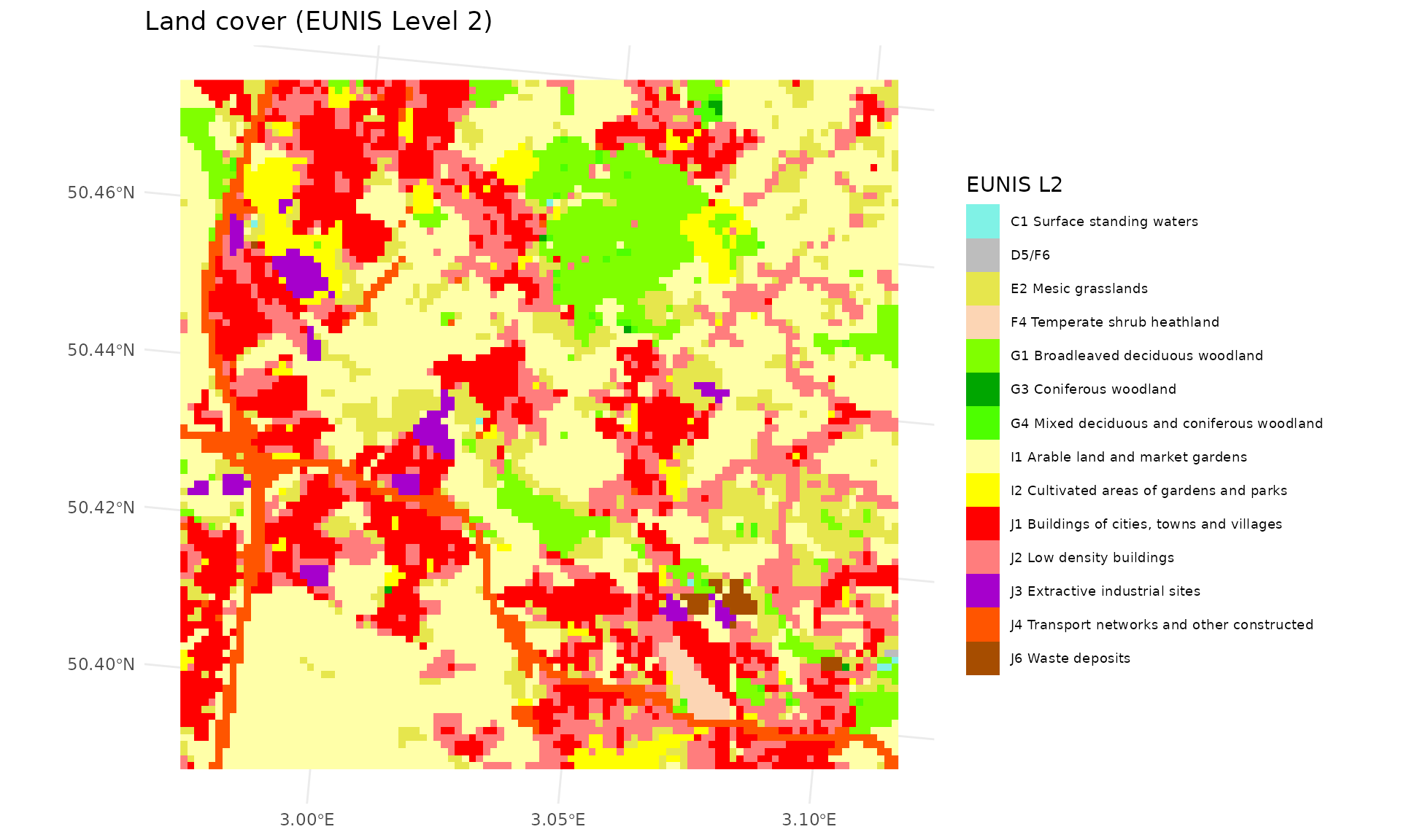

From species scores to rasters

The map is a raster, so the join is a reclassification. We write a small helper that replaces each EUNIS class by a species score. For combined codes such as "D5/F6", the scores of the two classes are averaged.

eunis_species_raster <- function(lc, species, var = "suitability",
                                 dict = eunis_species_dict) {
  lv <- terra::levels(lc)[[1]]
  names(lv) <- c("value", "code")
  d <- dict[dict$species_name == species, ]
  if (nrow(d) == 0) stop("Species not found: ", species)
  val <- vapply(strsplit(lv$code, "/"),
                function(cc) mean(d[[var]][match(cc, d$code_eunis)]), numeric(1))
  r <- lc
  levels(r) <- NULL                       # drop categories, keep pixel ids
  out <- terra::classify(r, cbind(lv$value, val))
  names(out) <- var
  out
}

vars <- c("suitability", "weight_breeding", "weight_foraging", "resistance")
microtus_eunis <- rast(lapply(vars, function(v) eunis_species_raster(eunis_lc, "Microtus_arvalis", v)))

p_score <- ggplot() +
  geom_spatraster(data = microtus_eunis[[1:3]]) +
  facet_wrap(~lyr) +
  scale_fill_gradient(low = "#ffffe5", high = "#004529", limits = c(0, 10),
                      na.value = "transparent", name = "Score") +
  theme_void()
p_res <- ggplot() +
  geom_spatraster(data = microtus_eunis[["resistance"]]) +
  scale_fill_gradient(low = "#fff5f0", high = "#67000d", trans = "log10", limits = c(1, 100),
                      na.value = "transparent", name = "Resistance") +
  theme_void() +
  labs(title = "resistance (1–100, log scale)")

p_score / p_res + plot_annotation(title = "Microtus arvalis – habitat layers from EUNIS")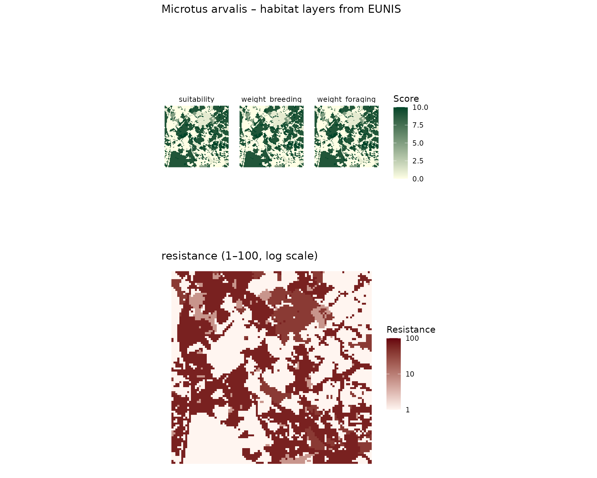

Scores of the classes present on the site

species <- c("Apodemus_sylvaticus", "Microtus_arvalis", "Myodes_glareolus",
             "Sorex_araneus", "Crocidura_russula", "Turdus_merula", "Passer_domesticus")
present <- unlist(strsplit(lv$code, "/"))

eunis_species_dict %>%
  filter(species_name %in% species, code_eunis %in% present) %>%
  left_join(ref_l2, by = c("code_eunis" = "code")) %>%
  mutate(species_name = gsub("_", " ", species_name),
         label = paste(code_eunis, substr(nomenclature, 1, 30))) %>%
  ggplot(aes(species_name, label, fill = suitability)) +
  geom_tile(colour = "white") +
  geom_text(aes(label = suitability), size = 3) +
  scale_fill_gradient(low = "#ffffe5", high = "#004529", limits = c(0, 10)) +
  theme_minimal() +
  theme(axis.text.x = element_text(angle = 30, hjust = 1, face = "italic")) +
  labs(x = NULL, y = NULL, fill = "Suitability",
       title = "Suitability of the EUNIS classes present at Metaleurop")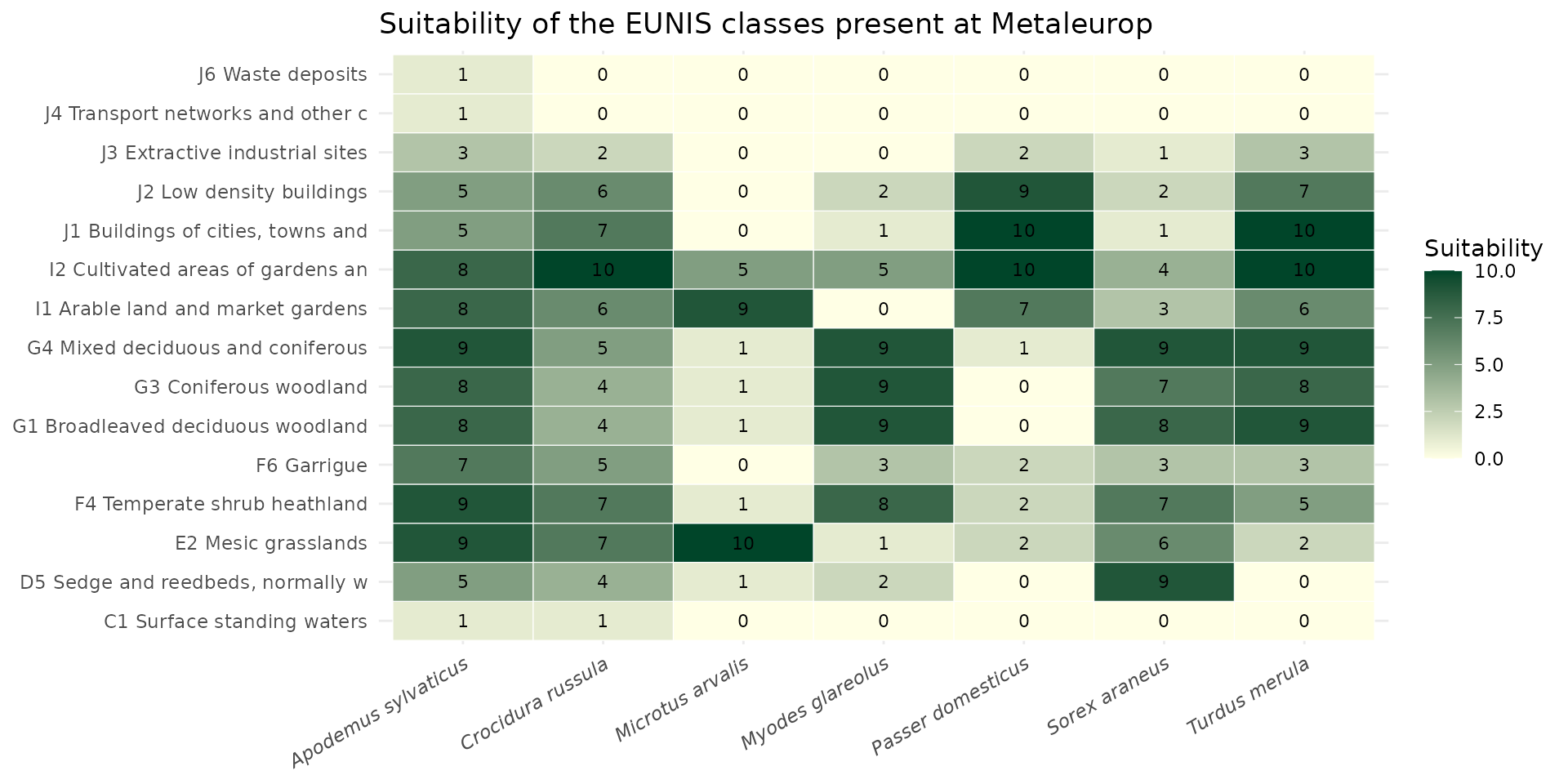

Arable land (I1), mesic grassland (E2) and gardens and parks (I2) are three separate classes here, with clearly different values for the two voles and the shrews. In OCS-GE they are a single cover.

Moving between nomenclatures

The OCS-GE / EUNIS crosswalk

OCS-GE and EUNIS do not nest: one describes what covers the ground, the other describes habitats. ref_ocsge_eunis gives, for each OCS-GE cover and for each (cover, use) pair that deserves it, a ranked list of EUNIS classes.

data("ref_ocsge_eunis")

# default EUNIS class of each cover, with the other candidates
ref_ocsge_eunis %>%
  filter(is.na(code_us)) %>%
  group_by(code_cs) %>%
  summarise(default = code_eunis[rank == 1],
            others = paste(code_eunis[rank > 1], collapse = ", ")) %>%
  left_join(ref_ocsge[, c("code_cs", "nomenclature")], by = "code_cs") %>%
  select(code_cs, nomenclature, default, others)
#> # A tibble: 14 × 4
#>    code_cs   nomenclature                            default others             
#>    <chr>     <chr>                                   <chr>   <chr>              
#>  1 CS1.1.1.1 Zones bâties                            J1      "J2"               
#>  2 CS1.1.1.2 Zones non bâties                        J4      "J1, J2"           
#>  3 CS1.1.2.1 Matériaux minéraux                      J4      "J3, J1, J6, H5"   
#>  4 CS1.1.2.2 Matériaux composites                    J6      ""                 
#>  5 CS1.2.1   Sols nus                                H5      "H3, H2, B1, B2, B…
#>  6 CS1.2.2   Surfaces d'eau                          C1      "C2, J5, C3"       
#>  7 CS1.2.3   Névés et glaciers                       H4      ""                 
#>  8 CS2.1.1.1 Feuillus                                G1      "G2, G5"           
#>  9 CS2.1.1.2 Conifères                               G3      "G5"               
#> 10 CS2.1.1.3 Mixte                                   G4      "G5"               
#> 11 CS2.1.2   Formations arbustives, sous-arbrisseaux F3      "F4, F5, F6, F9, F…
#> 12 CS2.1.3   Autres formations ligneuses             FB      ""                 
#> 13 CS2.2.1   Formations herbacées                    I1      "E2, I2, E1, E3, E…
#> 14 CS2.2.2   Autres formations non ligneuses         D1      "D2, D4, F1, D3"

Rows with a code_us refine the match, for instance for herbaceous cover:

ref_ocsge_eunis %>%
  filter(code_cs == "CS2.2.1", !is.na(code_us), rank <= 2) %>%
  select(code_us, rank, code_eunis, pct_metaleurop, note) %>%
  knitr::kable()

code_us	rank	code_eunis	pct_metaleurop	note
US1.1	1	I1	76	Arable crops. Crops and permanent grassland share this cover and use: the RPG (Registre Parcellaire Graphique) is needed to separate them
US1.1	2	E2	14	Permanent pastures and hay meadows
US1.2	1	G5	NA	Clear-cuts, forest rides and firebreaks (recently felled woodland)
US1.2	2	E2	NA
US1.3	1	J3	NA	Grassed parts of extraction sites
US1.3	2	E2	NA
US2	1	E2	14	Lawns of industrial sites (EUNIS E2.6)
US2	2	I2	1
US3	1	I2	32	Parks, sports grounds, cemeteries, campuses
US3	2	E2	15	Sports fields and large lawns (EUNIS E2.6)
US5	1	I2	1	Domestic gardens
US5	2	E2	5
US235	1	I2	NA	Gardens and green spaces of mixed urban areas
US235	2	E2	NA
US4.1.1	1	E2	9	Road verges and embankments
US4.1.1	2	J4	47
US4.1.2	1	E2	NA	Railway verges and embankments
US4.1.2	2	J4	NA
US4.1.3	1	E2	NA	Airfield grass
US4.1.3	2	J4	NA
US4.2	1	E2	9	Lawns of logistics sites
US4.3	1	E2	NA	Grass of utility networks (power-line corridors, dykes, basins)
US6.2	1	E2	NA	Abandoned grassland and herbaceous wasteland
US6.2	2	I1	NA	Recently abandoned arable land (EUNIS I1.5)
US6.3	1	E2	24	Unmanaged grassland. The grassland type (dry, mesic, wet, alpine) needs soil moisture or altitude data
US6.3	2	E1	0

rank is an expert reading of the two nomenclatures. pct_metaleurop is a measurement: the share of the area of each OCS-GE group that falls in the EUNIS class on this site. The two do not always agree, because of the 100 m pixel of the EUNIS map: gardens (US5) are I2 by definition, but they are too small to be the dominant class of a pixel, which is then classified as buildings.

The column main_cs gives the opposite direction, the main OCS-GE cover of each EUNIS class:

ref_ocsge_eunis %>%
  filter(main_cs) %>%
  group_by(code_cs) %>%
  summarise(eunis = paste(code_eunis, collapse = ", "))
#> # A tibble: 14 × 2
#>    code_cs   eunis                                             
#>    <chr>     <chr>                                             
#>  1 CS1.1.1.1 J1, J2                                            
#>  2 CS1.1.1.2 J4                                                
#>  3 CS1.1.2.1 J3                                                
#>  4 CS1.1.2.2 J6                                                
#>  5 CS1.2.1   H5, H3, H2, B1, B2, B3                            
#>  6 CS1.2.2   C1, C2, J5                                        
#>  7 CS1.2.3   H4                                                
#>  8 CS2.1.1.1 G1, G2, G5                                        
#>  9 CS2.1.1.2 G3                                                
#> 10 CS2.1.1.3 G4                                                
#> 11 CS2.1.2   F3, F4, F5, F6, F9, F2, F7, F8                    
#> 12 CS2.1.3   FB                                                
#> 13 CS2.2.1   I1, E2, I2, E1, E3, E4, E7, D5, C3, D2, D4, D6, E6
#> 14 CS2.2.2   D1, F1, D3

Translating a map

The crosswalk translates OCS-GE polygons into EUNIS classes, taking the (cover, use) pair when it is listed and the cover otherwise. This gives a EUNIS map with the geometry of OCS-GE:

best <- ref_ocsge_eunis %>% filter(rank == 1)
with_us <- best$code_eunis[match(paste(ocsge_us_metaleurop$code_cs, ocsge_us_metaleurop$code_us),
                                 paste(best$code_cs, best$code_us))]
cs_only <- best$code_eunis[match(paste(ocsge_us_metaleurop$code_cs, NA),
                                 paste(best$code_cs, best$code_us))]
ocsge_as_eunis <- ocsge_us_metaleurop %>%
  mutate(code_eunis = ifelse(is.na(with_us), cs_only, with_us)) %>%
  left_join(ref_l2, by = c("code_eunis" = "code")) %>%
  mutate(eunis = paste(code_eunis, substr(nomenclature, 1, 40)))

ggplot(ocsge_as_eunis) +
  geom_sf(aes(fill = eunis), color = NA) +
  scale_fill_manual(values = setNames(ocsge_as_eunis$couleur, ocsge_as_eunis$eunis), name = "EUNIS L2") +
  theme_minimal() +
  theme(legend.text = element_text(size = 7)) +
  labs(title = "OCS-GE cover and use, translated into EUNIS Level 2")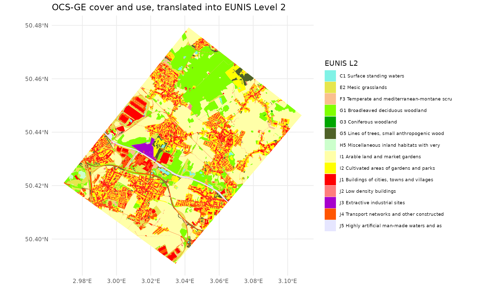

Compare with the EEA map above: the classes are the same, the grain is not.

Comparing the sources

To compare the three sources, we bring them onto the grid of the soil contamination raster (25 m).

ground_cd <- load_raster_extdata("ground_concentration_cd_compressed.tif")

ocsge_score_raster <- function(x, var = "suitability") {
  habitat_raster(ground_cd, habitat(x, habitat = TRUE, weight = x[[var]], touches = FALSE))
}
compare_sources <- function(species, var = "suitability") {
  cs <- join_ocsge_species(ocsge_us_metaleurop, species, us_col = NULL)
  us <- join_ocsge_species(ocsge_us_metaleurop, species)
  eu <- terra::project(eunis_species_raster(eunis_lc, species, var), ground_cd, method = "near")
  out <- c(ocsge_score_raster(cs, var), ocsge_score_raster(us, var), eu)
  names(out) <- c("OCS-GE cover", "OCS-GE cover and use", "EUNIS")
  # keep the pixels covered by the three sources
  terra::mask(out, terra::vect(sf::st_union(ocsge_us_metaleurop)))
}

plot_sources <- function(species) {
  ggplot() +
    geom_spatraster(data = compare_sources(species)) +
    facet_wrap(~lyr, ncol = 3) +
    scale_fill_gradient(low = "#ffffe5", high = "#004529", limits = c(0, 10),
                        na.value = "transparent", name = "Suitability") +
    theme_void() +
    labs(title = gsub("_", " ", species)) +
    theme(plot.title = element_text(face = "italic"))
}
plot_sources("Microtus_arvalis") / plot_sources("Myodes_glareolus") +
  plot_layout(guides = "collect")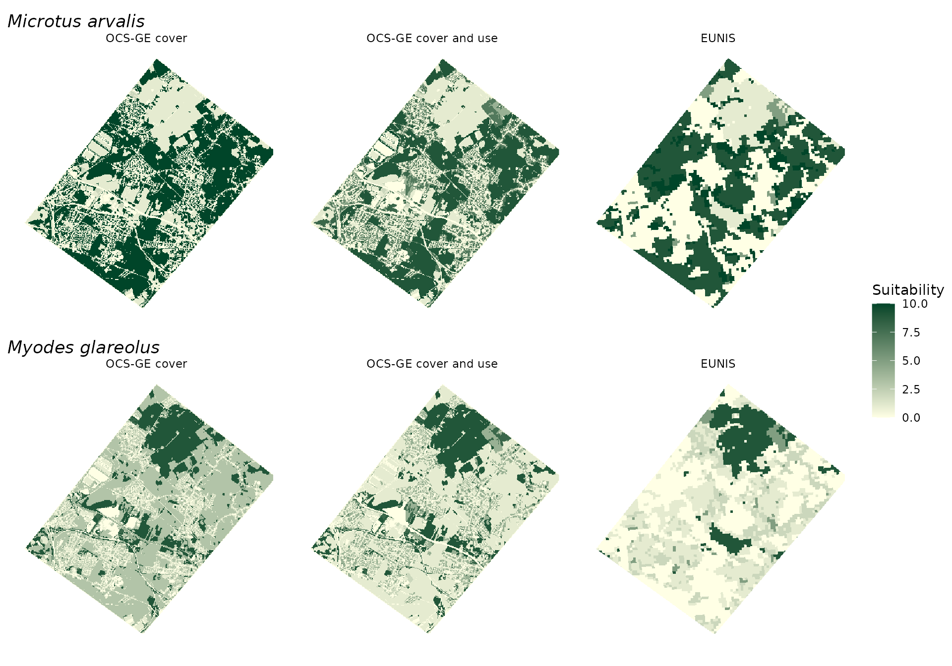

The table below gives, for a few species, the mean suitability of the site under each source and the correlation between the maps.

do.call(rbind, lapply(species, function(s) {
  v <- as.data.frame(compare_sources(s), na.rm = TRUE)
  data.frame(
    species = gsub("_", " ", s),
    mean_cover = round(mean(v[[1]]), 1),
    mean_cover_use = round(mean(v[[2]]), 1),
    mean_eunis = round(mean(v[[3]]), 1),
    cor_cover_vs_use = round(cor(v[[1]], v[[2]]), 2),
    cor_use_vs_eunis = round(cor(v[[2]], v[[3]]), 2)
  )
}))
#>               species mean_cover mean_cover_use mean_eunis cor_cover_vs_use
#> 1 Apodemus sylvaticus        6.7            6.7        6.8             0.98
#> 2    Microtus arvalis        5.6            4.8        4.7             0.98
#> 3    Myodes glareolus        3.6            2.9        1.8             0.93
#> 4       Sorex araneus        5.6            4.6        3.4             0.93
#> 5   Crocidura russula        5.3            5.4        5.9             0.79
#> 6       Turdus merula        6.1            5.5        6.6             0.78
#> 7   Passer domesticus        4.2            4.2        6.1             0.86
#>   cor_use_vs_eunis
#> 1             0.30
#> 2             0.43
#> 3             0.59
#> 4             0.51
#> 5             0.19
#> 6             0.25
#> 7             0.55

How to read it:

where the cover and the cover-and-use maps correlate strongly, the use adds little for this species on this site; where they do not, the species reacts to what the use separates (crops, gardens, clearings);
the correlation with EUNIS is never high. Part of the gap is thematic, and most of it is geometric: a 100 m pixel carries one class, while OCS-GE maps the fields, gardens and roads inside it.

Choosing a source

	OCS-GE cover	OCS-GE cover and use	EUNIS
Study area	France	France	Europe (EEA-39)
Smallest mapped object	a few meters	a few meters	100 m pixel
Built-up areas, roads	yes	yes	merged at 100 m
Crops, gardens, verges, clearings	one class	separated by the use	separated, when larger than a pixel
Crops versus permanent grassland	no	no	yes
Wetlands, grassland types, dunes	no	no	yes
Scores	scored for each cover	derived from EUNIS scores through `ref_ocsge_eunis`	scored for each class

In practice, for a French site of a few kilometers, OCS-GE with the use is the default choice, and EUNIS is worth overlaying where wetlands or grassland types matter for the species. Outside France, EUNIS is the only one of the three.

Other sources

The three sources above leave gaps that other geographic data can fill. None of them is wired into spacemodR yet; this section lists what each would bring, so that the same recipe (a map, a dictionary, a join) can be extended.

Source	What it would resolve	How it would enter
RPG (Registre Parcellaire Graphique, agricultural parcels)	Crops versus permanent grassland, and the crop type, inside `CS2.2.1` x `US1.1`	Splits a class: the parcel gives the EUNIS class (`I1`, `E2`, …) instead of the crosswalk
Wetland inventories, soil moisture	Wetlands (`D`) and wet grasslands (`E3`), which OCS-GE does not identify	Splits a class
Vegetation indices (NDVI and time series)	Vegetation density and phenology within a class: bare field or standing crop, mown or tall grass	Modulates a score within a class
LiDAR (canopy height, understorey, micro-topography)	Vegetation structure: hedges, young or mature stands, shrub layer	Modulates a score, or splits woodland and scrub classes
Topography (altitude, slope, aspect)	Alpine and subalpine classes, dry or wet slopes	Splits a class

Two kinds of data appear in this table. Those that split a class fit the current design directly: they only change which dictionary row a polygon or a pixel takes, as the land use does in join_ocsge_species(). Those that modulate a score are continuous, and need a rule to combine them with the class score (a multiplier between 0 and 1, for instance), which is specific to each species.

Toward connectivity

Whatever the source, the suitability raster is the source layer and the resistance raster is the resistance layer of compute_dispersal(method = "omniscape"). resistance is already on the 1–100 log scale in both dictionaries, so no transformation is needed. It must be at least 1: pixels outside the land cover map, left at 0 by habitat_raster(), have to be set to 1 or masked.

myodes <- join_ocsge_species(ocsge_us_metaleurop, "Myodes_glareolus")
src <- ocsge_score_raster(myodes, "suitability")
res <- ocsge_score_raster(myodes, "resistance")
res <- terra::ifel(res < 1, 1, res)

radius_px <- 500 / terra::res(ground_cd)[1]     # dispersal radius of 500 m
compute_dispersal(x = src, method = "omniscape",
                  options = list(resistance = res, radius = radius_px))

See Habitat Layer for building habitat objects with several layers, and Landscape Connectivity (Omniscape) for running and interpreting the connectivity model.

References

O’Connor, Louise MJ, Julien Renaud, Yue Dou, et al. 2024. “Habitat Suitability of European Land Systems for Terrestrial Vertebrates.” Global Ecology and Biogeography 33 (11): e13903.