Introduction
In this vignette, we explore the database linking OCS-GE (French GIS layer for Occupation du Sol à Grande Échelle) labels with species labels.
We will analyze how different land cover types act as habitats with varying qualities or resistances for different species, starting with the Wood mouse (Apodemus sylvaticus).
The database construction
To build the habitat database for spacemod, we transitioned from traditional static mapping to a dynamic semantic analysis. Here is a breakdown of how this new methodology compares to previous standards.
The Original Framework (O’Connor et al., 2024 ; @oconnor2024habitat)
The foundational method described by O’Connor et al. (2024) relies on an “expert-based” crosswalk to define optimal habitats for European terrestrial vertebrates. It links a European land systems map—which accounts for both land cover and land use intensity—to standardized habitat classifications from GlobCover and the IUCN Red List. This approach assigns simple, discrete suitability scores: 2 for optimal habitat, 1 for secondary habitat, and 0 for unsuitable. These scores were then manually penalized by subtracting points if specific keywords related to land use intensity or threats (e.g., agricultural intensification) appeared in the species’ IUCN descriptions. Ultimately, this generated Area of Habitat (AOH) maps, filtering existing occurrence maps to show simple presence or absence at a 1 km² resolution.
The LLM-Assisted Approach for spacemod
Our approach steps away from rigid keyword matching and discrete scoring, moving toward a semantic analysis of a species’ ecological requirements.Instead of using the broad European land systems, this database utilizes the fine-scale French OCS-GE (Occupation du Sol à Grande Échelle) nomenclature. Each OCS-GE code was enriched with precise ecological context. For example, paved roads are described as creating a “barrier effect,” while mineral soils are noted as “thermophilic.”Using a Large Language Model (Gemini), we fed the AI free-text descriptions of both preferred and avoided habitats (sourced from EEA databases). The model conceptually analyzed these texts against our enriched OCS-GE descriptions.
Instead of a single presence/absence score, the model simultaneously
generates four continuous variables (on a scale of 0 to 10) that capture
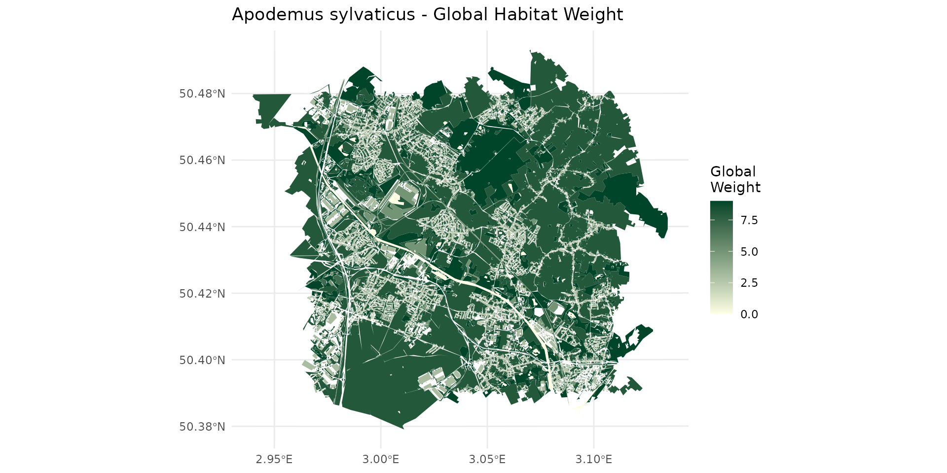
finer landscape ecology concepts: * weight_global: Overall
habitat suitability (closest to the traditional AOH score). *
weight_movement: Landscape permeability for species
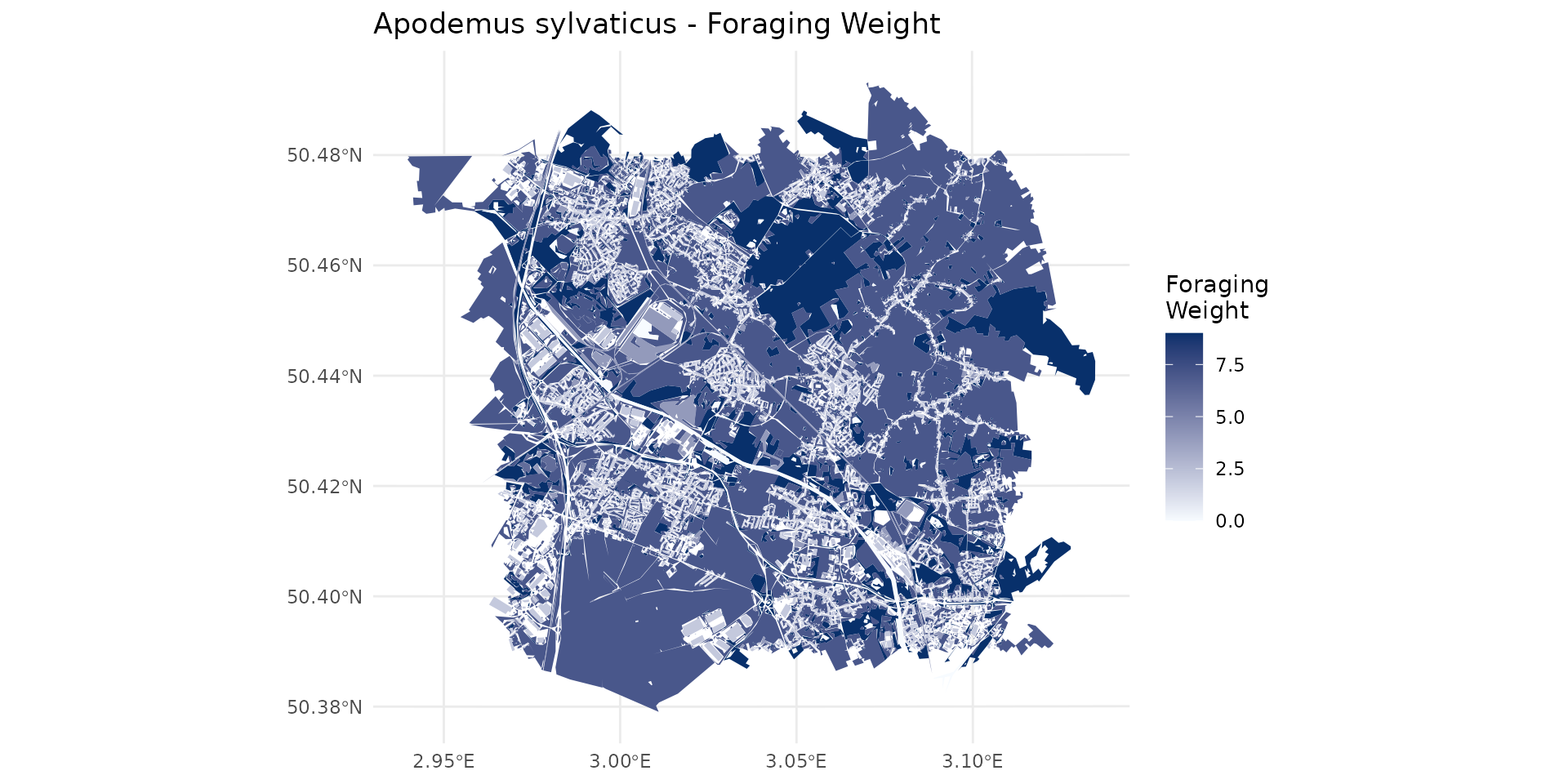
dispersion. * weight_foraging: Habitat attractiveness
specifically for feeding and resource acquisition. *
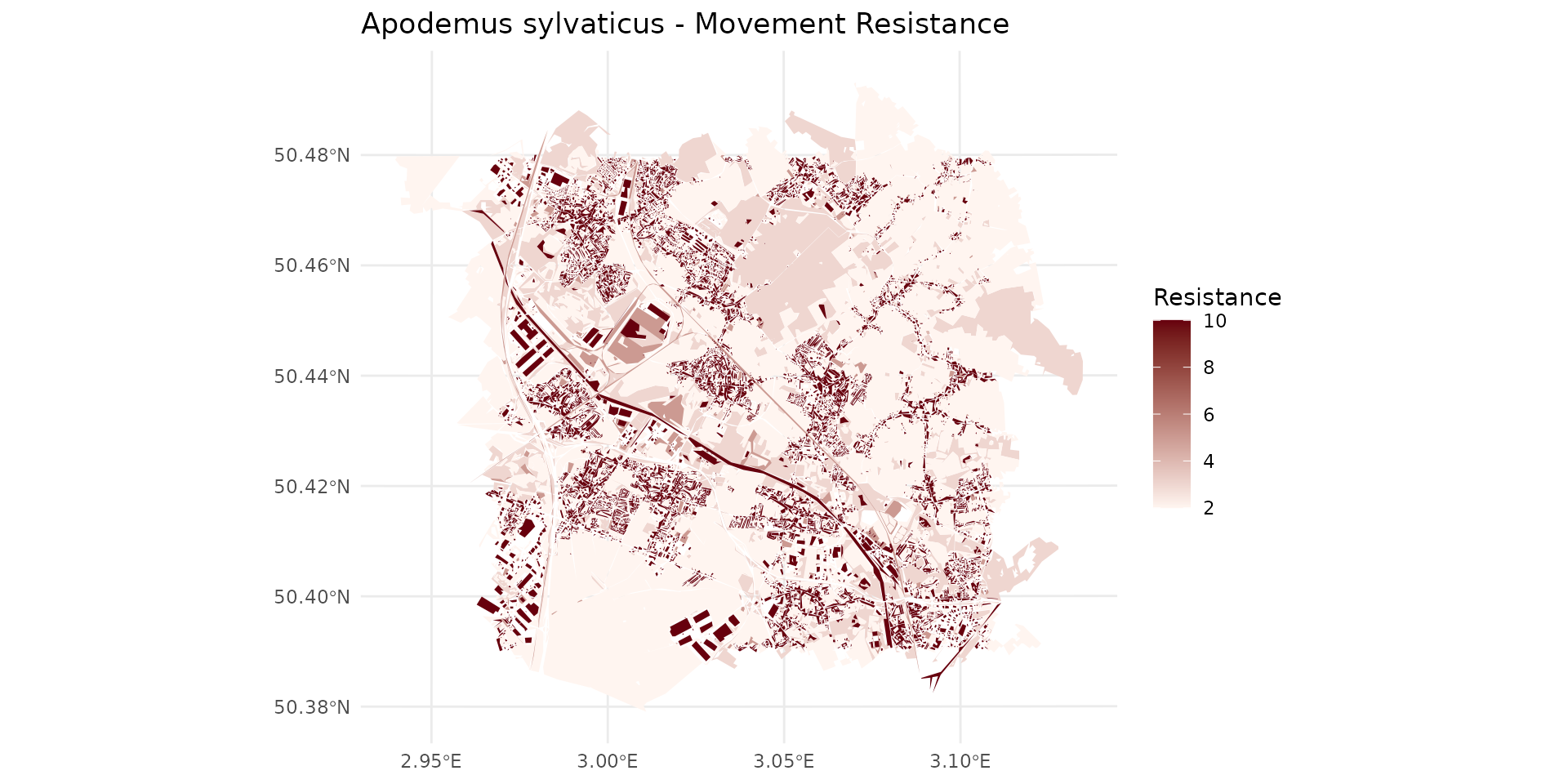
resistance: The impedance or barrier effect of the
environment, heavily informed by the “avoided-habitat” descriptions.
The Fundamental Difference
This new method represents a major shift in both scale and functionality. The original methodology relied on rigid keyword penalties to output a discrete matrix (0, 1, or 2), answering a simple question: can the species live in this pixel? By leveraging natural language understanding, our method generates a continuous matrix (0-10) that distinguishes between an environment where a species simply survives, one it actively seeks for food, and one it merely uses for transit. These variables are specifically designed to be injected into complex spatial ecological models (such as graph theory or Circuitscape), offering a much more nuanced view of landscape connectivity than traditional AOH mapping.
Defining Habitat
Weighted species habitat with OCS-GE layer for Apodemus sylvaticus
First, we load the necessary datasets provided by spacemodR:
- The species dictionary assigning weights to land cover codes.
- The OCS-GE nomenclature reference (containing names and specific hex colors).
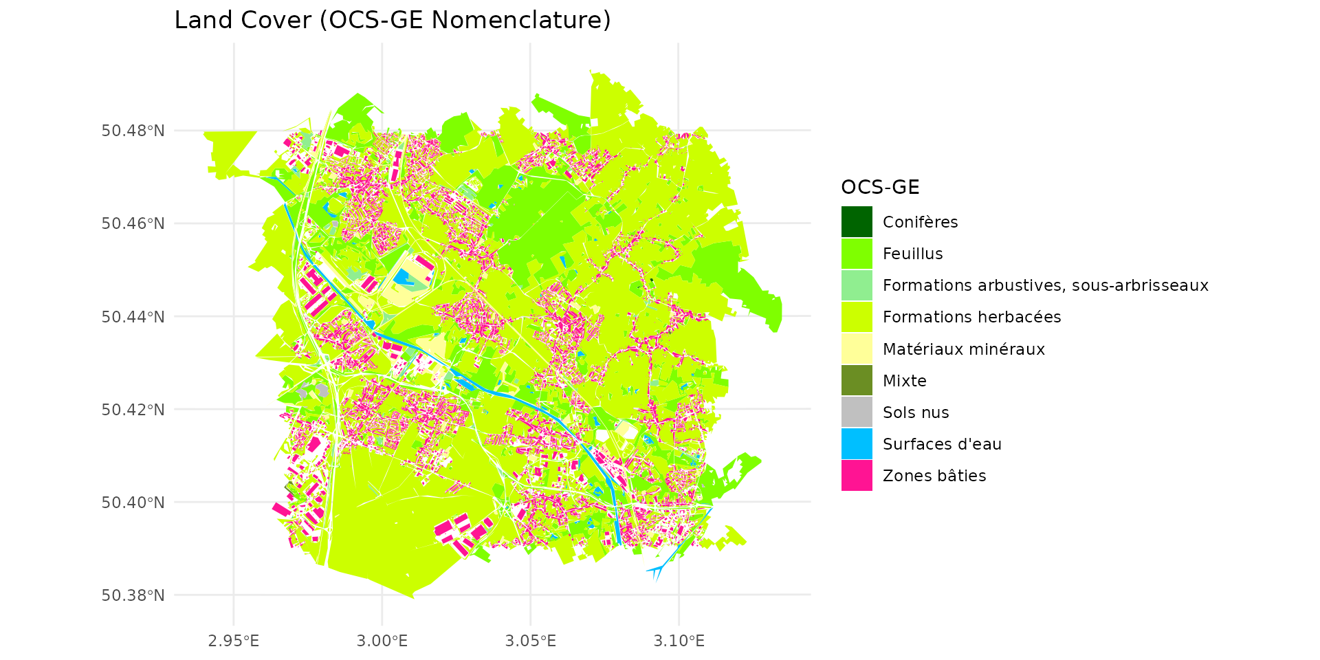
- The spatial layer for OCS-GE (here, we use the ocsge_metaleurop dataset as our base map).
# Load the species dict and reference tables
data("ocsge_species_dict")
data("ref_ocsge")
# Load spatial data
data("ocsge_metaleurop")
sf_ocsge <- ocsge_metaleuropWe filter our species dictionary for Apodemus sylvaticus and join it with the reference nomenclature to link the OCS-GE codes to their descriptive labels and predefined colors.
# Filter for Apodemus sylvaticus
dfhab_Apsy <- ocsge_species_dict[
grepl("Apodemus_sylvaticus",ocsge_species_dict$nom_espece, ignore.case = TRUE),
]
# Join ref_ocsge with the species dictionary.
# ref_ocsge$code_cs_ (with spaces) matches ocsge_species_dict$code_cs
df_merged_Apsy <- ref_ocsge %>%
dplyr::left_join(dfhab_Apsy, by = c("code_cs_" = "code_cs"))
# Join with the spatial sf object. Assuming sf_ocsge uses 'code_cs' (without spaces)
sf_Apsy <- sf_ocsge %>%
dplyr::left_join(df_merged_Apsy, by = "code_cs")Understanding Habitat Values
By examining the weight_global (wg), we can classify the landscape into different habitat qualities for the species:
- Non-habitat area (wg = 0):
df_merged_Apsy %>%
filter(weight_global == 0) %>%
pull(nomenclature) %>%
unique()
#> [1] "Surfaces d'eau" "Névés et glaciers"- Very Poor habitat (0 < wg <= 3):
df_merged_Apsy %>%
filter(weight_global > 0, weight_global <= 3) %>%
pull(nomenclature) %>%
unique()
#> [1] "Zones bâties" "Zones non bâties"
#> [3] "Autres formations non ligneuses"- Poor habitat (3 < wg <= 7):
df_merged_Apsy %>%
filter(weight_global > 7) %>%
pull(nomenclature) %>%
unique()
#> [1] "Feuillus"
#> [2] "Conifères"
#> [3] "Mixte"
#> [4] "Formations arbustives, sous-arbrisseaux"
#> [5] "Formations herbacées"- Good habitat (wg > 7):