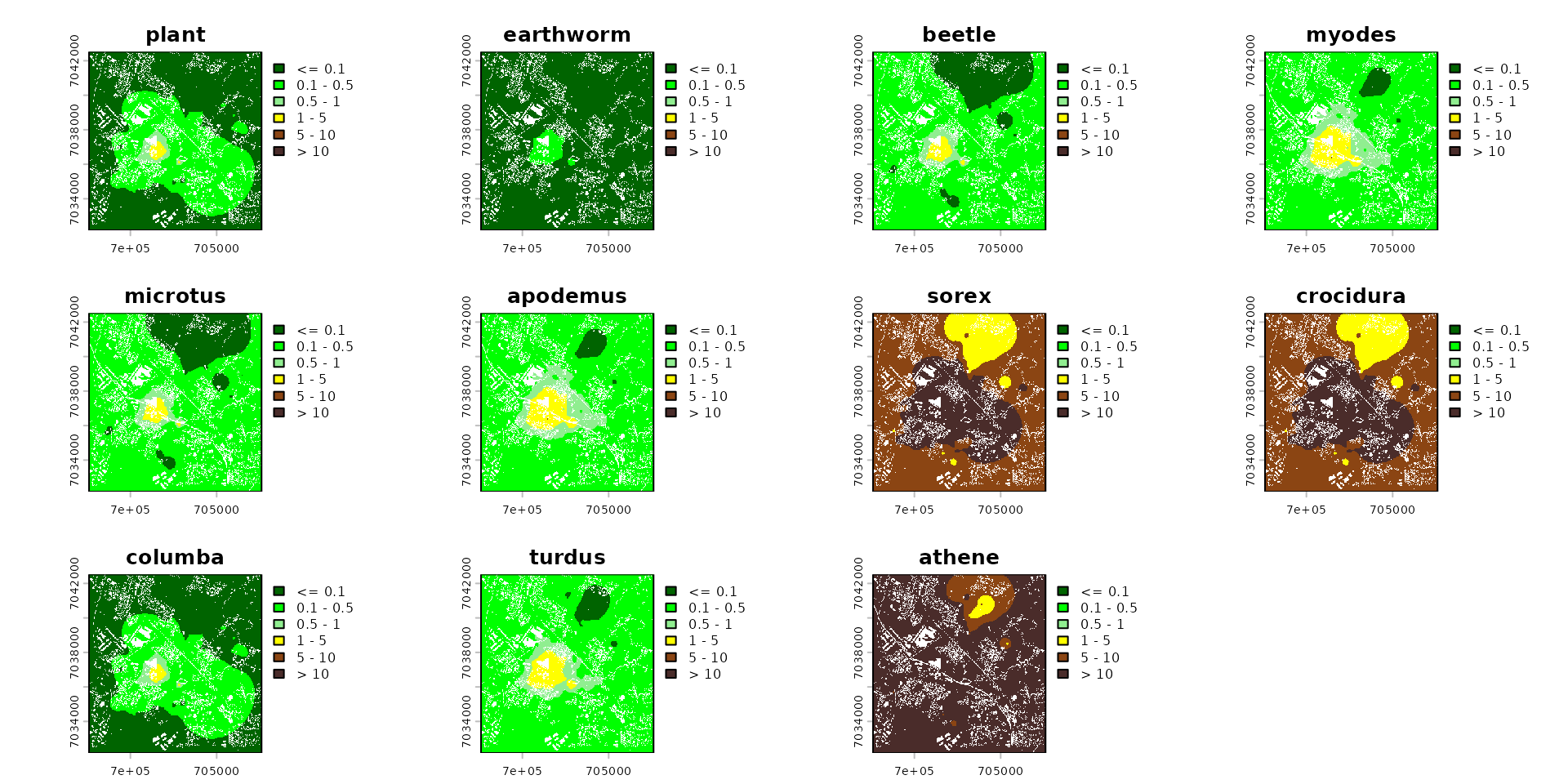
Berisp-like: a trophic model of contamination

library(spacemodR)
library(rstan)
library(ggplot2)
library(scales)
library(stringr)
library(dplyr)
library(tidyr)
library(terra)
library(purrr)

Trophic web

Often, in other notebooks, we started by defining the habitats. But in this case, let’s begin by defining the species and their trophic relationships.

The goal is to reproduce the results of the Berisp model by using the same species. Here are the species we want to model:

The soil category: although not a species, we need this layer to account for areas with and without soil. This allows us to isolate the kriging process used to estimate contamination, which we will address later. Note that we could also define layers for pH and Organic Matter (%OM), which are sometimes included in transfer equations.

Next, the organisms directly linked to the soil:

Plants (aka plant): let’s include all plants (trees, grasses, cereal crops, and shrubs). We could break down this stratum further, but let’s keep it simple.
Earthworms (aka earthworm: we will use this single category to represent soil invertebrates.
Ground beetles, (aka beetle): a highly species-rich family present everywhere. They are strongly influenced by soil conditions and occasionally prey on earthworms.

Mammals. We are only considering small mammals:

Bank vole (Myodes glareolus, aka myodes): a strictly herbivorous rodent that prefers wooded habitats.
Common vole (Microtus arvalis, aka microtus): a highly herbivorous rodent that primarily inhabits meadows.
Wood mouse (Apodemus sylvaticus, aka apodemus): a rodent with a more diverse diet than the previous two.
Shrew (aka shrew, Soricidae: Sorex araneus and the greater white-toothed shrew, Crocidura russula): classified as insectivores, they feed on ground beetles, but also consume earthworms and slugs.

Finally, 3 bird species (Note: le texte original disait “2” mais en liste 3):

Pigeon/Dove (aka columba): not included in Berisp, but useful as a common herbivore/granivore; it is widely used in Eco-SSL and various exposure models.
Blackbird (Turdus merula, aka turdus): an omnivore that feeds on insects, earthworms, very small animals, and seeds.
Little owl (Athene noctua, aka athene): feeds heavily on insects, earthworms, and small mammals. This will be the apex predator of our food web.

Plants and Beetles

So, let’s start creating the food web.

For plants and earthworm, 100% of the feeding behavior is based on soil. We keep thing simples, so we do not make any assumption on other sources of contaminantion, and we could eventually modulate the intake rate with the flux equatiosn comming after.

For ground beetles (Carabidae), according to recent literature (@sacco2024carabs and @deroulers2019carabs), ground beetles display a highly opportunistic and plastic diet, adapting their food intake based on environmental availability. While they are major predators of soil invertebrates like earthworms, they also exhibit a feeding continuum that includes a significant intake of weed seeds and plant material, particularly within specific tribes. To maintain simplicity within our food web model, we will bypass these highly dynamic seasonal shifts and assume a fixed dietary composition for the ground beetles consisting of 10% soil particles (accounting for incidental ingestion during foraging), 45% vegetation, and 45% earthworms.

trophic_df_init <- trophic() |>
  add_link("soil", "plant", 1) |>
  add_link("soil", "earthworm", 1)

# beetle and beetles
trophic_df <- trophic_df_init |>
  add_link("soil", "beetle", 0.1) |>
  add_link("plant", "beetle", 0.45) |>
  add_link("earthworm", "beetle", 0.45)

plot(trophic_df_init, colors = species_colors)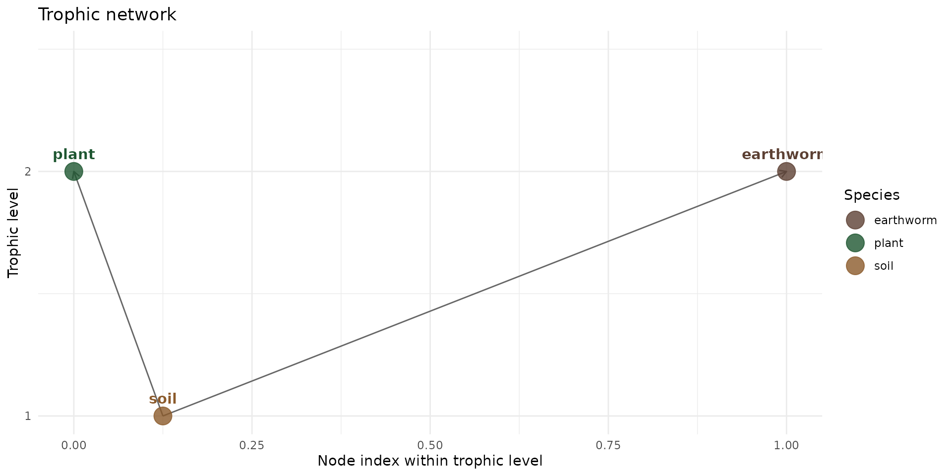

Diet of mammals and birds: the EltonTraits 1.0 database

Before going any further, we have two datasets from the EltonTraits 1.0 database, one for birds (9,994 species) and one for mammals (5,401 species), which will help us refine these dietary profiles. That is what we will explore here.

data("DBFunc_MamFuncDat")
data("DBFunc_BirdFuncDat")

head(DBFunc_MamFuncDat)
#>   MSW3_ID               Scientific    MSWFamilyLatin Diet.Inv Diet.Vend
#> 1       1   Tachyglossus aculeatus    Tachyglossidae      100         0
#> 2       2  Zaglossus attenboroughi    Tachyglossidae      100         0
#> 3       3        Zaglossus bartoni    Tachyglossidae      100         0
#> 4       4        Zaglossus bruijni    Tachyglossidae      100         0
#> 5       5 Ornithorhynchus anatinus Ornithorhynchidae       80         0
#> 6       6      Caluromys philander       Didelphidae       20         0
#>   Diet.Vect Diet.Vfish Diet.Vunk Diet.Scav Diet.Fruit Diet.Nect Diet.Seed
#> 1         0          0         0         0          0         0         0
#> 2         0          0         0         0          0         0         0
#> 3         0          0         0         0          0         0         0
#> 4         0          0         0         0          0         0         0
#> 5         0         20         0         0          0         0         0
#> 6         0          0        10         0         20         0        10
#>   Diet.PlantO Diet.Source Diet.Certainty ForStrat.Value ForStrat.Certainty
#> 1           0       Ref_1            ABC              G                  A
#> 2           0      Ref_65            ABC              G                  A
#> 3           0       Ref_2             D1              G                  A
#> 4           0       Ref_1            ABC              G                  A
#> 5           0       Ref_1            ABC              G                  A
#> 6          40       Ref_1            ABC             Ar                  A
#>   ForStrat.Comment Activity.Nocturnal Activity.Crepuscular Activity.Diurnal
#> 1                                   1                    1                0
#> 2                                   1                    0                0
#> 3                                   1                    0                0
#> 4                                   1                    0                0
#> 5                                   1                    1                1
#> 6                                   1                    1                0
#>   Activity.Source Activity.Certainty BodyMass.Value BodyMass.Source
#> 1           Ref_1                ABC        3025.00         Ref_117
#> 2           Ref_1                ABC        8532.39    Ref_2, Ref_3
#> 3           Ref_1                ABC        7180.00         Ref_131
#> 4           Ref_1                ABC       10139.50         Ref_117
#> 5           Ref_1                ABC        1484.25         Ref_117
#> 6           Ref_1                ABC         229.25         Ref_117
#>   BodyMass.SpecLevel
#> 1                  1
#> 2                  0
#> 3                  1
#> 4                  1
#> 5                  1
#> 6                  1

Concise Diet Descriptions (EltonTraits 1.0):

Diet.PlantO: % of other vegetative tissues (leaves, stems, roots, bark).
Diet.Fruit: % of fruits and berries consumed.
Diet.Seed: % of seeds, nuts, grains, or cones.
Diet.Nect: % of nectar, pollen, or plant exudates.
Diet.Inv: % of invertebrates (insects, larves, worms, mollusks).
Diet.Vfish: % of fish consumed.
Diet.Vect: % of ectothermic vertebrates (reptiles and amphibians).
Diet.Vend: % of endothermic vertebrates (birds and mammals).
Diet.Scav: % of scavenging activity (eating carrion/dead animals).
Diet.Vunk: % of unknown or unclassified vertebrates.

And also:

Diet.Source: Reference/ID of the scientific data source.
Diet.Certainty: Data certainty score (direct species study vs. genus-level extrapolation).

Small mammals: voles and shrew

diet_mammal <- DBFunc_MamFuncDat |>
  dplyr::filter(
    Scientific %in% 
      c("Microtus arvalis", "Myodes glareolus", "Apodemus sylvaticus", "Sorex araneus", "Crocidura russula")
    )

# transform data_set
species_short = c(
  "Microtus arvalis"="microtus",
  "Myodes glareolus"="myodes",
  "Apodemus sylvaticus"="apodemus",
  "Sorex araneus"="sorex",
  "Crocidura russula"="crocidura")
diet_long <- diet_mammal |>
  pivot_longer(
    cols = c(Diet.Inv, Diet.Vend, Diet.Vect, Diet.Vfish, Diet.Vunk, 
             Diet.Scav, Diet.Fruit, Diet.Nect, Diet.Seed, Diet.PlantO),
    names_to = "Diet_Category",
    values_to = "Value"
  ) |>
  mutate(
    Diet_Category = stringr::str_remove(Diet_Category, "Diet\\."),
    Diet_Category = factor(Diet_Category, levels = trophic_order),
    Species_Short = species_short[Scientific]
  )

# create plot
ggplot(diet_long, aes(x = Diet_Category, y = Value, color = Species_Short, shape=Scientific)) +
  geom_point(size = 3, alpha = 0.8, position = position_jitter(width = 0.15, height = 0)) +
  theme_minimal(base_size = 14) +
  scale_color_manual(values = species_colors) +
  labs(
    title = "Dietary composition of some small-mammals species",
    x = "Diet Category",
    y = "Percentage / Value",
    color = "Species"
  ) +
  theme(
    axis.text.x = element_text(angle = 45, hjust = 1),
    panel.grid.minor = element_blank(),
  )

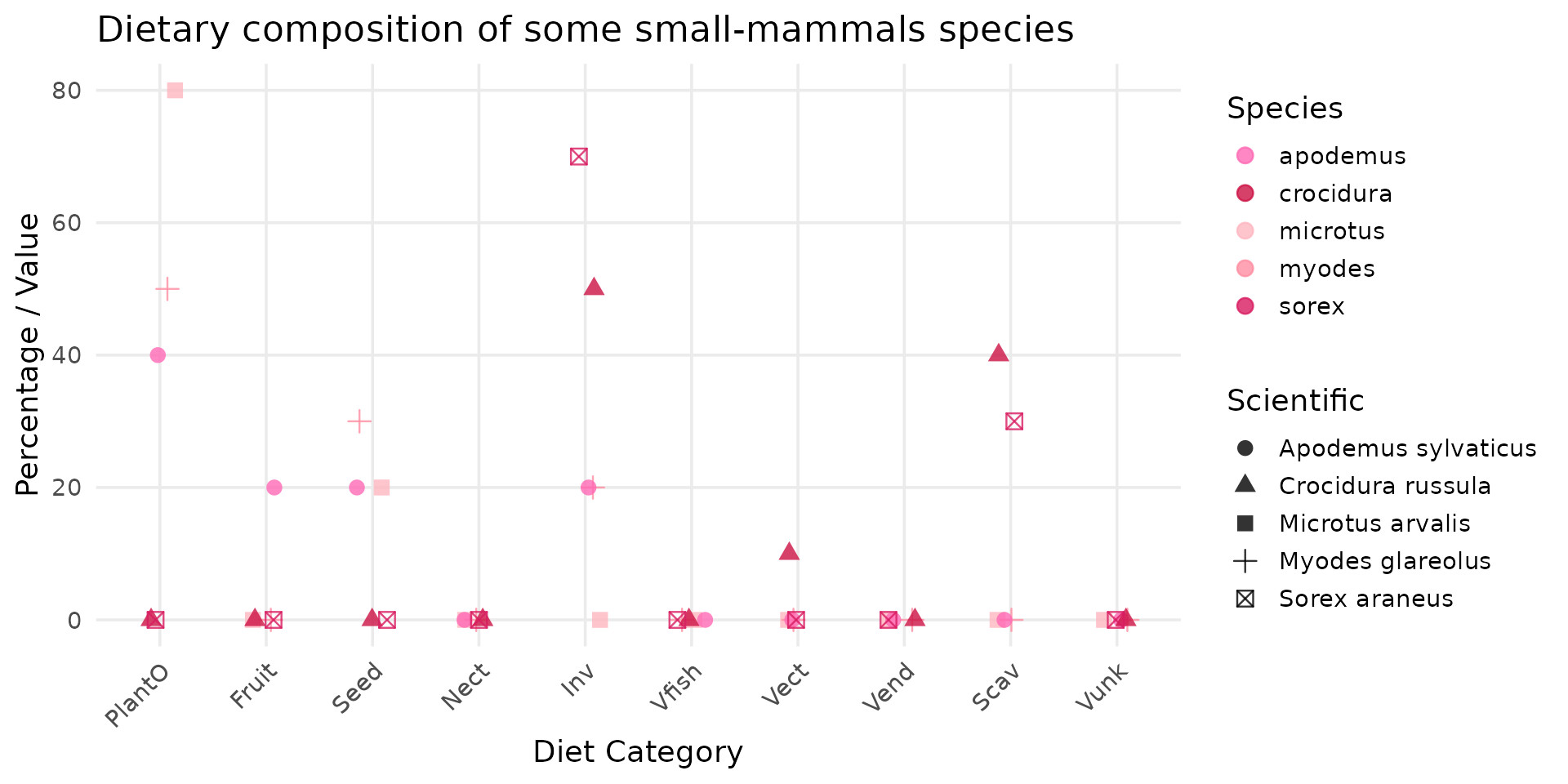
We can compared the results with what is used in the Berisp documentation, and see that the results are similar:

	grass	herbs	berries	seeds	earthworm	beetle	soil
bank vole (Myodes glareolus)	20	20	26	24	4	4	2
common vole (Microtus arvalis)	42	41		15			2
wood mouse (Apodemus sylvaticus)	6	6	12	58	8	8	2
shrew (Sorex araneus or Crocidura russula)					49	49	2

So we add mammals to the trophic network

trophic_df <- trophic_df |>
  # myodes
  add_link("soil", "myodes", 0.02) |>
  add_link("plant", "myodes", 0.9) |>
  add_link("earthworm", "myodes", 0.04) |>
  add_link("beetle", "myodes", 0.04) |>
  # microtus
  add_link("soil", "microtus", 0.02) |>
  add_link("plant", "microtus", 0.98) |>
  # wood mouse
  add_link("soil", "apodemus", 0.02) |>
  add_link("plant", "apodemus", 0.82) |>
  add_link("earthworm", "apodemus", 0.08) |>
  add_link("beetle", "apodemus", 0.08) |>
  # sorex
  add_link("soil", "sorex", 0.02) |>
  add_link("earthworm", "sorex", 0.49) |>
  add_link("beetle", "sorex", 0.49) |>
  # crocidura
  add_link("soil", "crocidura", 0.02) |>
  add_link("earthworm", "crocidura", 0.49) |>
  add_link("beetle", "crocidura", 0.49)

plot(trophic_df, colors = species_colors)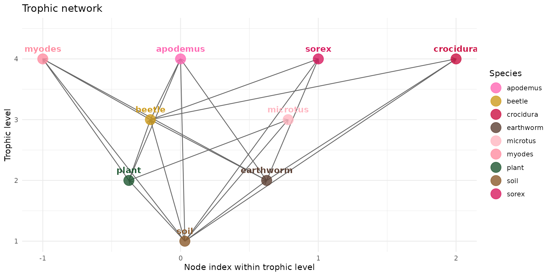

Birds: little owl and black bird

diet_bird <- DBFunc_BirdFuncDat |>
  dplyr::filter(
    Scientific %in% 
      c("Athene noctua", "Turdus merula", "Columba palumbus")
    )

# transform data_set
species_short = c(
  "Columba palumbus"="columba",
  "Athene noctua"="athene",
  "Turdus merula"="turdus")
diet_long <- diet_bird |>
  pivot_longer(
    cols = c(Diet.Inv, Diet.Vend, Diet.Vect, Diet.Vfish, Diet.Vunk, 
             Diet.Scav, Diet.Fruit, Diet.Nect, Diet.Seed, Diet.PlantO),
    names_to = "Diet_Category",
    values_to = "Value"
  ) |>
  mutate(
    Diet_Category = stringr::str_remove(Diet_Category, "Diet\\."),
    Diet_Category = factor(Diet_Category, levels = trophic_order),
    Species_Short = species_short[Scientific]
  )

# create plot
ggplot(diet_long, aes(x = Diet_Category, y = Value, color = Species_Short, shape=Scientific)) +
  geom_point(size = 3, alpha = 0.6, position = position_jitter(width = 0.15, height = 0)) +
  theme_minimal(base_size = 14) +
  scale_color_manual(values = species_colors) +
  labs(
    title = "Dietary composition of some small-mammals species",
    x = "Diet Category",
    y = "Percentage / Value",
    color = "Species"
  ) +
  theme(
    axis.text.x = element_text(angle = 45, hjust = 1),
    panel.grid.minor = element_blank(),
  )

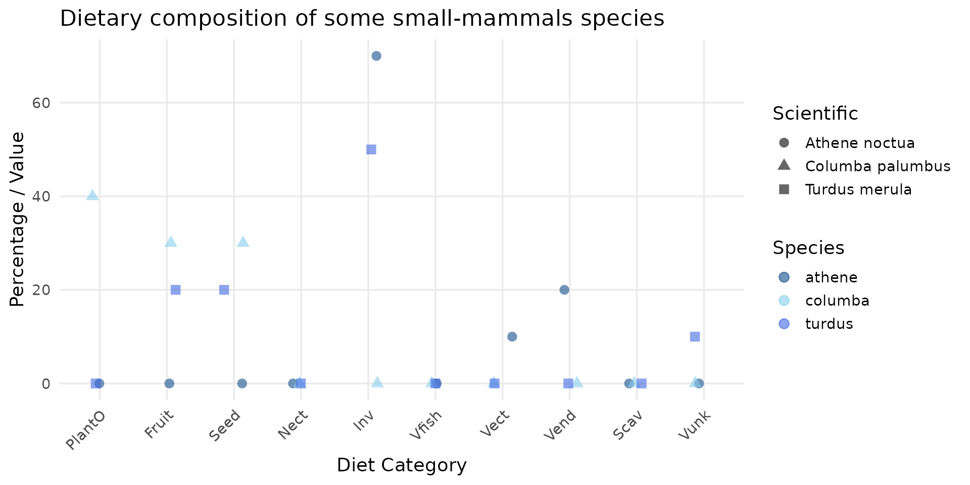
From this graph, we observe the following:

Columba palumbus is strictly herbivorous/granivorous, consisting of 40% plants, 30% fruits, and 30% seeds.
Turdus merula is more of an omnivore, with 20% fruits, 20% seeds, and 50% invertebrates (which we will divide equally between earthworms and beetles). The remaining 10% consists of unknown vertebrates (likely because they are not consumed whole), which we will not take into account.
Athene noctua feeds on 70% invertebrates (which we will split into 35% earthworms and 35% beetles), 20% endotherms, and 10% ectotherms (we will distribute this combined 30% across all organisms).

And we finally add birds to the trophic network:

trophic_df <- trophic_df |>
  # columba
  add_link("plant", "columba", 1) |>
  # turdus
  add_link("plant", "turdus", 0.4) |>
  add_link("earthworm", "turdus", 0.3) |>
  add_link("beetle", "turdus", 0.3) |>
  # athene
  add_link("earthworm", "athene", 0.35) |>
  add_link("beetle", "athene", 0.35) |>
  add_link("myodes", "athene", 0.06) |>
  add_link("microtus", "athene", 0.06) |>
  add_link("apodemus", "athene", 0.06) |>
  add_link("sorex", "athene", 0.06) |>
  add_link("crocidura", "athene", 0.06)

plot(trophic_df, colors = species_colors, edge_width="norm_target")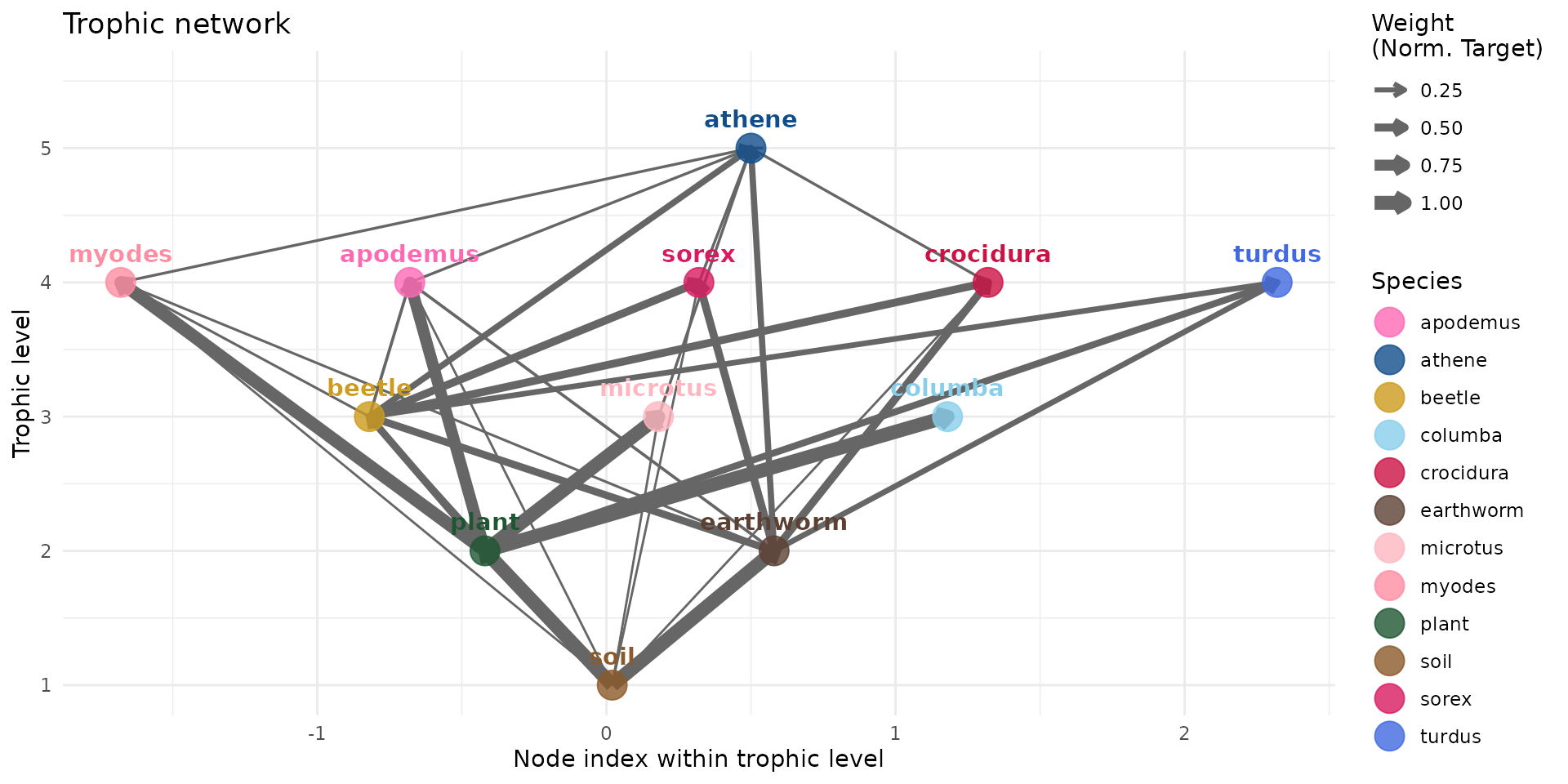

Food Ingestion Rate per Body Weight

We have the energy needs of 749 species, 97 mammals, 107 birds, 170 fishes, 51 reptiles, 11 amphibians, 110 crustacean, 65 arthropods, 75 protozoa

data("FmrBT")

close species

The list is missing some species.

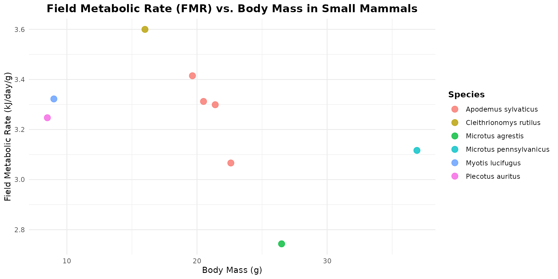
Sorex and Crocidura (Shrews): the list lacks true shrews (Soricidae). When seeking a metabolic surrogate for temperate shrews (Sorex spp.) within this dataset, small temperate insectivorous bats, such as Myotis lucifugus and Plecotus auritus, serve as excellent physiological equivalents. Like true shrews, these bats are lightweight (often weighing between 5 and 12 grams) and operate under immense thermal pressure from temperate and boreal climates. Because they are strictly insectivorous, they share a highly active foraging strategy that demands a continuous supply of high-protein, easily digestible prey. Most importantly, the extreme energetic cost of flapping flight combined with their tiny body size forces these bats to run a hyper-metabolic “engine.”
Myodes glareolus (Bank Vole): the list is highly enriched with rodents that are phylogenetically very close to the bank vole. Most notably, Cleithrionomys rutilus belongs to the exact same genus (as Myodes and Cleithrionomys are synonymous in modern taxonomy). Additionally, species from the genera Microtus (like M. agrestis and M. pennsylvanicus) and Arvicola belong to the same family, Cricetidae, sharing identical microtine (vole-like) metabolic and toxicokinetic traits.

energy_mammal <- FmrBT |>
  filter(
    SpeciesVerbatim %in% c(
      "Apodemus sylvaticus", "Plecotus auritus", "Myotis lucifugus",
      "Cleithrionomys rutilus",
      "Microtus agrestis", "Microtus pennsylvanicus")
  )

# plot
ggplot(data = energy_mammal, aes(x = Mass_g, y = FMR_kJ_d/Mass_g, color = SpeciesVerbatim)) +
  geom_point(size = 3.5, alpha = 0.8) + 
  labs(
    title = "Field Metabolic Rate (FMR) vs. Body Mass in Small Mammals",
    x = "Body Mass (g)",
    y = "Field Metabolic Rate (kJ/day/g)",
    color = "Species"
  ) +
  theme_minimal() +
  theme(
    plot.title = element_text(face = "bold", size = 14, hjust = 0.5),
    legend.title = element_text(face = "bold"),
    legend.position = "right"
  )

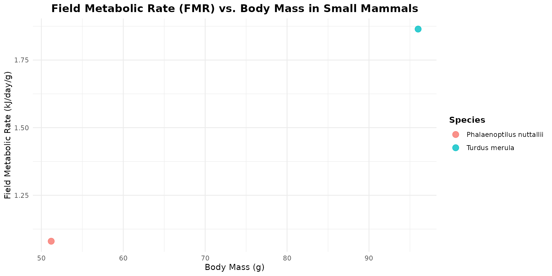
Athene noctua (Little Owl): true owls (Strigiformes) are completely absent from this dataset. The closest relative available is Phalaenoptilus nuttallii (the common poorwill), which belongs to the Caprimulgiformes (nightjars). While it is a distinct family, nightjars share a nocturnal, insectivorous niche with small owls and belong to the same broader evolutionary landbird/Strisores lineage, making it the best available surrogate for nocturnal avian traits.

energy_mammal <- FmrBT |>
  filter(SpeciesVerbatim %in% c(
      "Turdus merula", "Phalaenoptilus nuttallii")
  )

# plot
ggplot(data = energy_mammal, aes(x = Mass_g, y = FMR_kJ_d/Mass_g, color = SpeciesVerbatim)) +
  geom_point(size = 3.5, alpha = 0.8) + 
  labs(
    title = "Field Metabolic Rate (FMR) vs. Body Mass in Small Mammals",
    x = "Body Mass (g)",
    y = "Field Metabolic Rate (kJ/day/g)",
    color = "Species"
  ) +
  theme_minimal() +
  theme(
    plot.title = element_text(face = "bold", size = 14, hjust = 0.5),
    legend.title = element_text(face = "bold"),
    legend.position = "right"
  )

FIR weighted

library(tibble)

species_traits <- tribble(
  ~species,    ~bw,          ~FIRbw,  # En-têtes des colonnes (précédées d'un tilde ~)
  # --- INSECTES ---
  "beetle",    55 * 10^-3,   0.51,    # bw: Zygmunt et al. 2006 / FIR: Pocock et al. 2020
  # --- MAMMIFÈRES ---
  "myodes",    20,           0.3,     # bw & FIR: à vérifier
  "microtus",  25,           0.45,    # bw & FIR: à vérifier
  "apodemus",  21.7,         0.206,   # bw & FIR: POLARIS
  "sorex",     9.7,          13.3,    # bw & FIR: POLARIS
  "crocidura", 11.6,         13.3,    # bw: à vérifier / FIR: POLARIS sur Sorex
  # --- OISEAUX ---
  "columba",   490,          0.074,   # bw & FIR: POLARIS - Tier 2
  "turdus",    113,          0.5,     # FIR: POLARIS - Tier 2 (between seeds 0.185 & slugs 1.01)
  "athene",    180,          0.30     # bw & FIR: à vérifier
)
species_traits <- as.data.frame(species_traits)
# Calcul automatique du FIR absolu (Food Ingestion Rate en g/jour)
species_traits$FIR <- species_traits$FIRbw * species_traits$bw
# Création des vecteurs nommés pour la suite du modèle
vec_FIRbw <- setNames(species_traits$FIRbw, species_traits$species)
vec_FIR   <- setNames(species_traits$FIR, species_traits$species)

trophic_df_FIR <- trophic_df_init |>
  # Invertébrés
  add_link("soil", "beetle", 0.1 * vec_FIR["beetle"]) |>
  add_link("plant", "beetle", 0.45 * vec_FIR["beetle"]) |>
  add_link("earthworm", "beetle", 0.45 * vec_FIR["beetle"] ) |>
  # Mammifères - Myodes
  add_link("soil", "myodes", 0.02 * vec_FIR["myodes"]) |>
  add_link("plant", "myodes", 0.9 * vec_FIR["myodes"]) |>
  add_link("earthworm", "myodes", 0.04 * vec_FIR["myodes"]) |>
  add_link("beetle", "myodes", 0.04 * vec_FIR["myodes"]) |>
  # Mammifères - Microtus
  add_link("soil", "microtus", 0.02 * vec_FIR["microtus"]) |>
  add_link("plant", "microtus", 0.98 * vec_FIR["microtus"]) |>
  # Mammifères - Apodemus
  add_link("soil", "apodemus", 0.02 * vec_FIR["apodemus"]) |>
  add_link("plant", "apodemus", 0.82 * vec_FIR["apodemus"]) |>
  add_link("earthworm", "apodemus", 0.08 * vec_FIR["apodemus"]) |>
  add_link("beetle", "apodemus", 0.08 * vec_FIR["apodemus"]) |>
  # Mammifères - Musaraignes
  add_link("soil", "sorex", 0.02 * vec_FIR["sorex"]) |>
  add_link("earthworm", "sorex", 0.49 * vec_FIR["sorex"]) |>
  add_link("beetle", "sorex", 0.49 * vec_FIR["sorex"]) |>
  add_link("soil", "crocidura", 0.02 * vec_FIR["crocidura"]) |>
  add_link("earthworm", "crocidura", 0.49 * vec_FIR["crocidura"]) |>
  add_link("beetle", "crocidura", 0.49 * vec_FIR["crocidura"]) |>
  # Oiseaux
  add_link("plant", "columba", 1 * vec_FIR["columba"]) |>
  add_link("plant", "turdus", 0.4 * vec_FIR["turdus"]) |>
  add_link("earthworm", "turdus", 0.3 * vec_FIR["turdus"]) |>
  add_link("beetle", "turdus", 0.3 * vec_FIR["turdus"]) |>
  # Super-Prédateur - Athene
  add_link("earthworm", "athene", 0.35 * vec_FIR["athene"]) |>
  add_link("beetle", "athene", 0.35 * vec_FIR["athene"]) |>
  add_link("myodes", "athene", 0.06 * vec_FIR["athene"]) |>
  add_link("microtus", "athene", 0.06 * vec_FIR["athene"]) |>
  add_link("apodemus", "athene", 0.06 * vec_FIR["athene"]) |>
  add_link("sorex", "athene", 0.06 * vec_FIR["athene"]) |>
  add_link("crocidura", "athene", 0.06 * vec_FIR["athene"])

We can normalize on target (sum to 1 for each target/to node):

plot(trophic_df_FIR, colors = species_colors, edge_width="norm_target")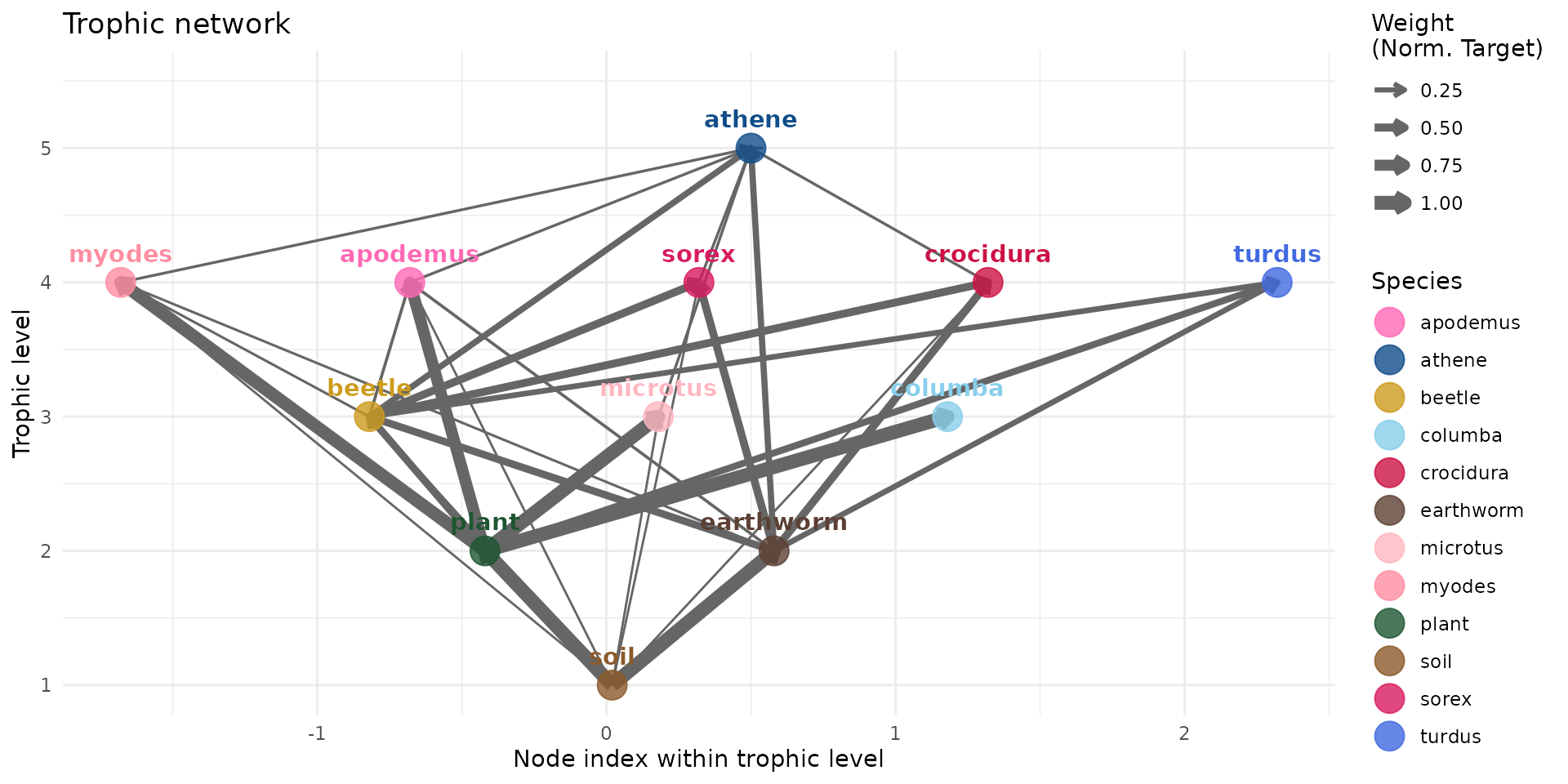

or we can normalize for the whole graph (uses the raw weights).

plot(trophic_df_FIR, colors = species_colors, edge_width="raw")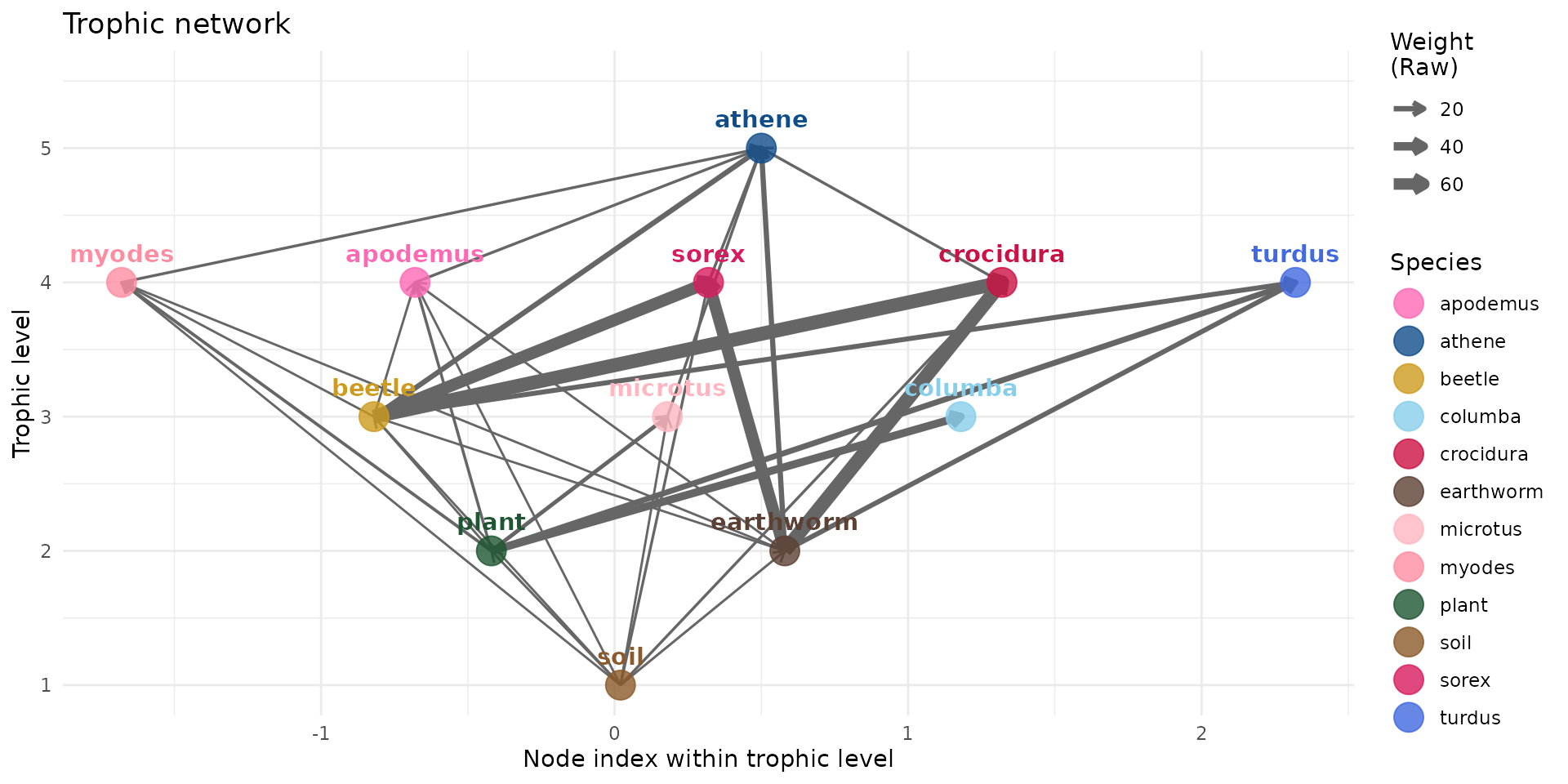

Here we have the daily food ingestion rate per body weight (FIRbw).

And we see that shrews having a high FIRbw, would as have a strong potential intake rate of the contaminant.

trophic_df_FIRbw <- trophic_df_init |>
  # beetle
  add_link("soil", "beetle", 0.1 * vec_FIRbw["beetle"]) |>
  add_link("plant", "beetle", 0.45 * vec_FIRbw["beetle"]) |>
  add_link("earthworm", "beetle", 0.45 * vec_FIRbw["beetle"]) |>
  # myodes
  add_link("soil", "myodes", 0.02 * vec_FIRbw["myodes"]) |>
  add_link("plant", "myodes", 0.9 * vec_FIRbw["myodes"]) |>
  add_link("earthworm", "myodes", 0.04 * vec_FIRbw["myodes"]) |>
  add_link("beetle", "myodes", 0.04 * vec_FIRbw["myodes"]) |>
  # microtus
  add_link("soil", "microtus", 0.02 * vec_FIRbw["microtus"]) |>
  add_link("plant", "microtus", 0.98 * vec_FIRbw["microtus"]) |>
  # wood mouse (apodemus)
  add_link("soil", "apodemus", 0.02 * vec_FIRbw["apodemus"]) |>
  add_link("plant", "apodemus", 0.82 * vec_FIRbw["apodemus"]) |>
  add_link("earthworm", "apodemus", 0.08 * vec_FIRbw["apodemus"]) |>
  add_link("beetle", "apodemus", 0.08 * vec_FIRbw["apodemus"]) |>
  # sorex
  add_link("soil", "sorex", 0.02 * vec_FIRbw["sorex"]) |>
  add_link("earthworm", "sorex", 0.49 * vec_FIRbw["sorex"]) |>
  add_link("beetle", "sorex", 0.49 * vec_FIRbw["sorex"]) |>
  # crocidura
  add_link("soil", "crocidura", 0.02 * vec_FIRbw["crocidura"]) |>
  add_link("earthworm", "crocidura", 0.49 * vec_FIRbw["crocidura"]) |>
  add_link("beetle", "crocidura", 0.49 * vec_FIRbw["crocidura"]) |>
  # columba
  add_link("plant", "columba", 1 * vec_FIRbw["columba"]) |>
  # turdus
  add_link("plant", "turdus", 0.4 * vec_FIRbw["turdus"]) |>
  add_link("earthworm", "turdus", 0.3 * vec_FIRbw["turdus"]) |>
  add_link("beetle", "turdus", 0.3 * vec_FIRbw["turdus"]) |>
  # athene
  add_link("earthworm", "athene", 0.35 * vec_FIRbw["athene"]) |>
  add_link("beetle", "athene", 0.35 * vec_FIRbw["athene"]) |>
  add_link("myodes", "athene", 0.06 * vec_FIRbw["athene"]) |>
  add_link("microtus", "athene", 0.06 * vec_FIRbw["athene"]) |>
  add_link("apodemus", "athene", 0.06 * vec_FIRbw["athene"]) |>
  add_link("sorex", "athene", 0.06 * vec_FIRbw["athene"]) |>
  add_link("crocidura", "athene", 0.06 * vec_FIRbw["athene"])

plot(trophic_df_FIRbw, colors = species_colors, edge_width="raw")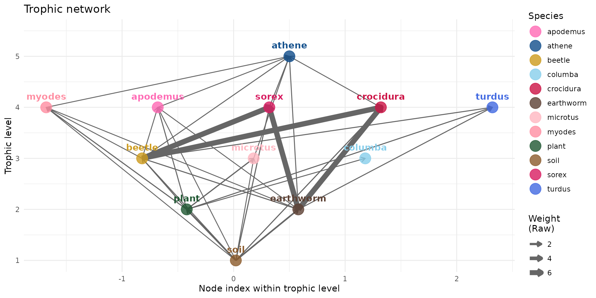

Habitat

Once again, we load data from a site in northern France.

Here, we use the provided data (ocsge_metaleurop and roi_metaleurop) along with the ggplot2 package for visualization.

# Load a study area (e.g., the Metaleurop site) and its land cover data
data("roi_metaleurop")
data("ocsge_metaleurop")

ggplot() +
  theme_minimal() +
  geom_sf(data=ocsge_metaleurop, aes(fill=code_cs), color=NA) +
  geom_sf(data=roi_metaleurop, fill=NA, color="red", size=1) +
  theme(legend.position = "none") +
  labs(title="Land Cover in the Region of Interest (ROI)")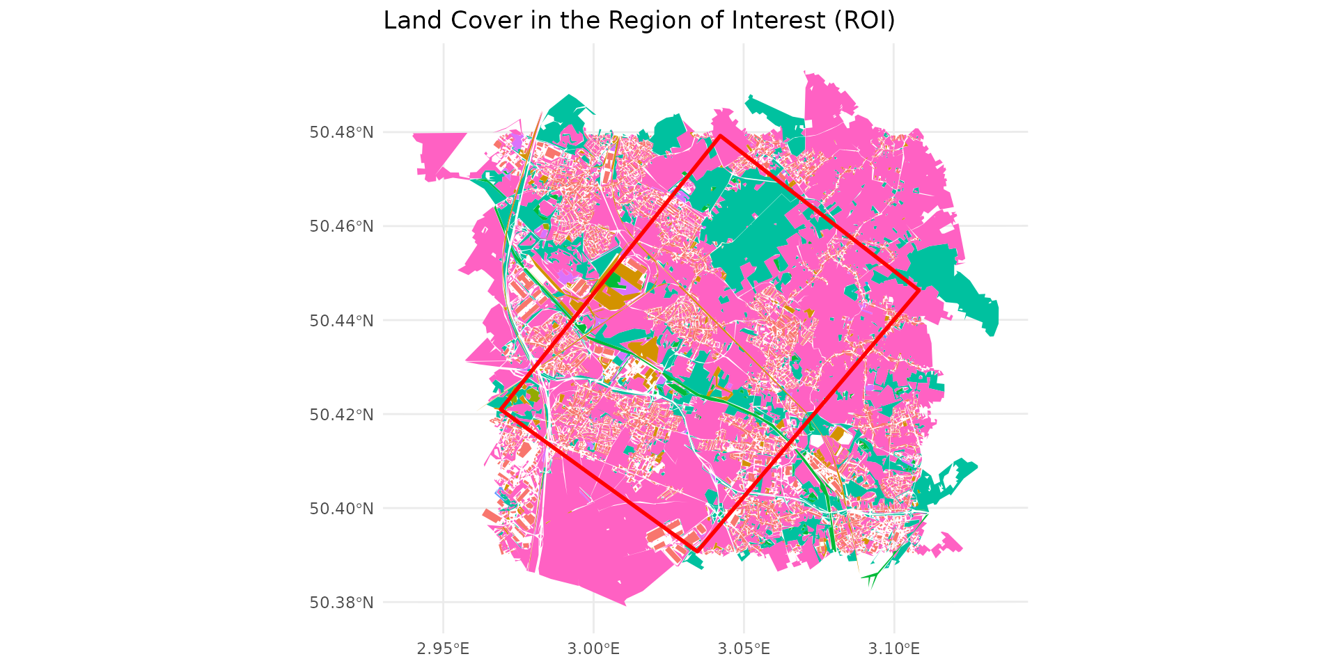

From these vector polygons, we define habitats for our species. A habitat is a combination of favorable, unfavorable, or neutral zones. These geometries are then rasterized (converted into regular grids) to prepare them for modeling.

# Habitat definition based on OSGE codes (which are in the `ocsge_metaleurop` table)
layer_soil_natural = ocsge_metaleurop$code_cs %in% 
  c("CS1.2.1","CS2.1.1.1","CS2.1.1.2","CS2.1.1.3", "CS2.1.2","CS2.1.3","CS2.2.1","CS2.2.3")
layer_soil_artificial = ocsge_metaleurop$code_cs %in%
  c("CS1.1.1.1", "CS1.1.1.2", "CS1.1.2.1")
layer_plant = ocsge_metaleurop$code_cs %in% 
   c("CS2.1.1.1", "CS2.1.1.2", "CS2.1.1.3", "CS2.1.3", "CS2.2.1")

habitat_soil = habitat() |>
  add_habitat(ocsge_metaleurop[layer_soil_natural,]) |>
  add_nohabitat(ocsge_metaleurop[layer_soil_artificial,])
plot(habitat_soil)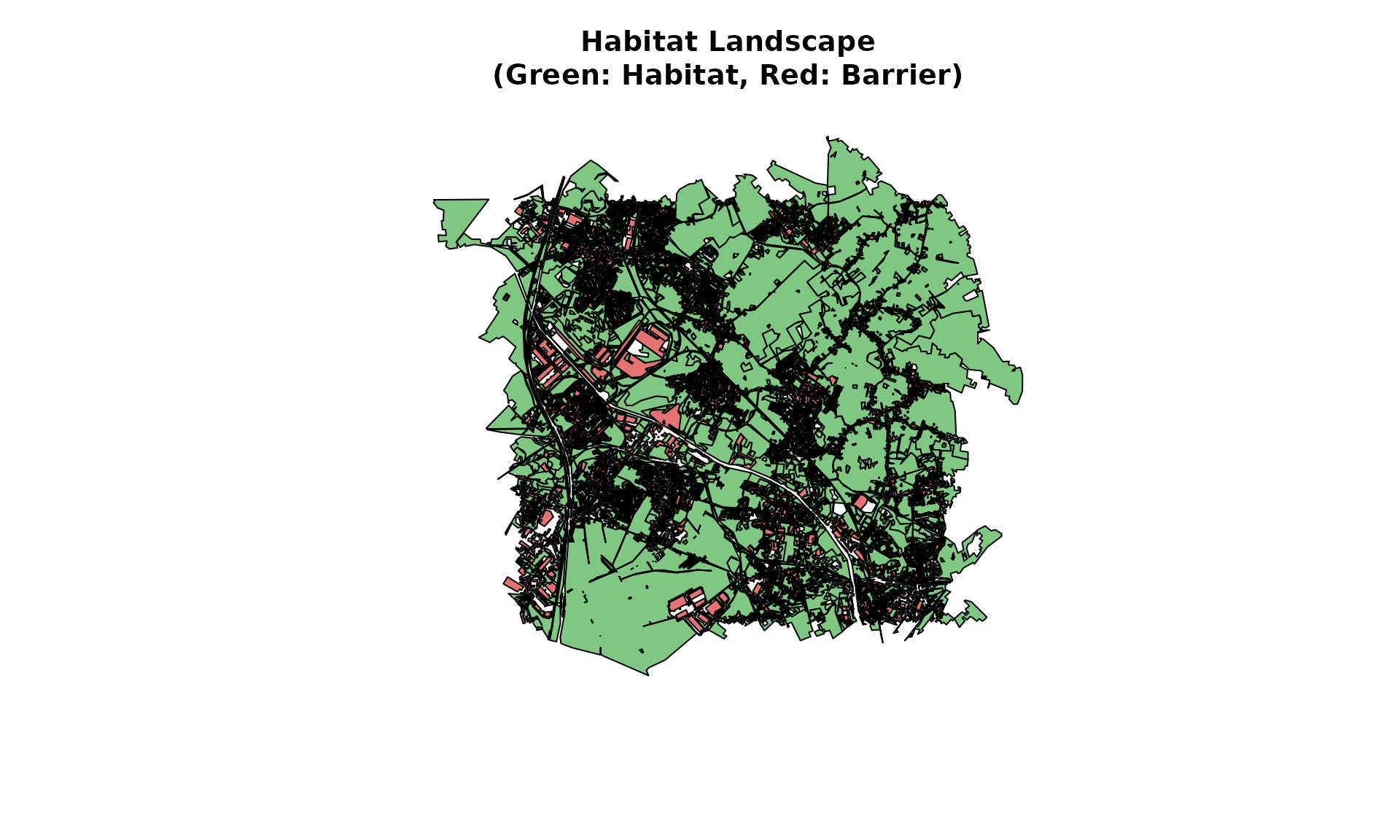

habitat_plant = habitat() |>
  add_habitat(ocsge_metaleurop[layer_plant,]) |>
  add_nohabitat(ocsge_metaleurop[layer_soil_artificial,])

We assume that earthworm and beetle have the same habitat that soil: everywhere there is soil, it is an habitat for earthworm and beetle.

habitat_earthworm = habitat_soil
habitat_beetle = habitat_soil

Database of Habitat base on @oconnor2024habitat

In this section, for birds and mammals we use the data base we build using LLM based on the original database created by @oconnor2024habitat where we linked species habitat to enriched OCS-GE descriptions. Then, instead of a single presence/absence score, the model simultaneously generates four continuous variables (on a scale of 0 to 10) that capture finer landscape ecology concepts: * weight_global: Overall habitat suitability (closest to the traditional AOH score). * weight_movement: Landscape permeability for species dispersion. * weight_foraging: Habitat attractiveness specifically for feeding and resource acquisition. * resistance: The impedance or barrier effect of the environment, heavily informed by the “avoided-habitat” descriptions.

data("ocsge_species_dict")

This database includes 935 species, including 499 birds, 215 mammals, 136 reptiles, and 85 amphibians.

For example, for the common vole (Microtus arvalis):

microtus_hab <- join_ocsge_species(ocsge_metaleurop, "Microtus_arvalis")
plot_species_habitat(microtus_hab)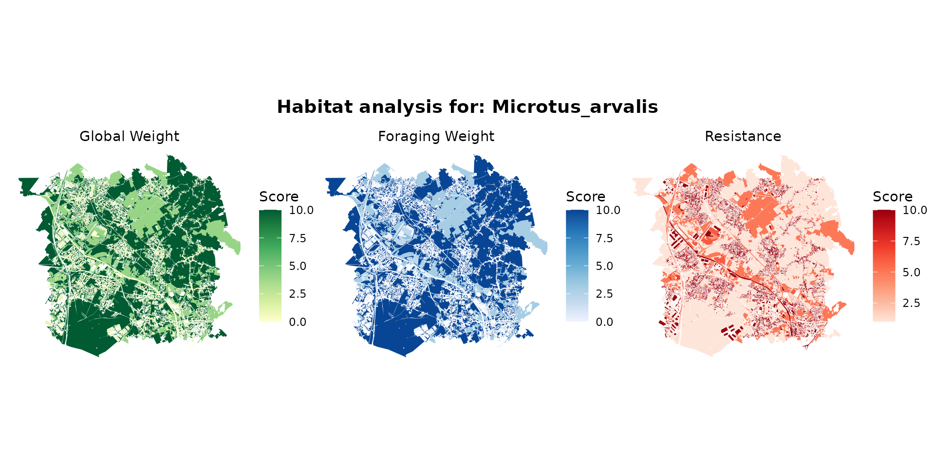

microtus_habitat <- habitat(microtus_hab, habitat=TRUE, weight=microtus_hab$weight_global) |>
  add_nohabitat(microtus_hab[microtus_hab$resistance==10,])
plot(microtus_habitat, main="Microtus arvalis, (green=habitat, red=non-habitat)")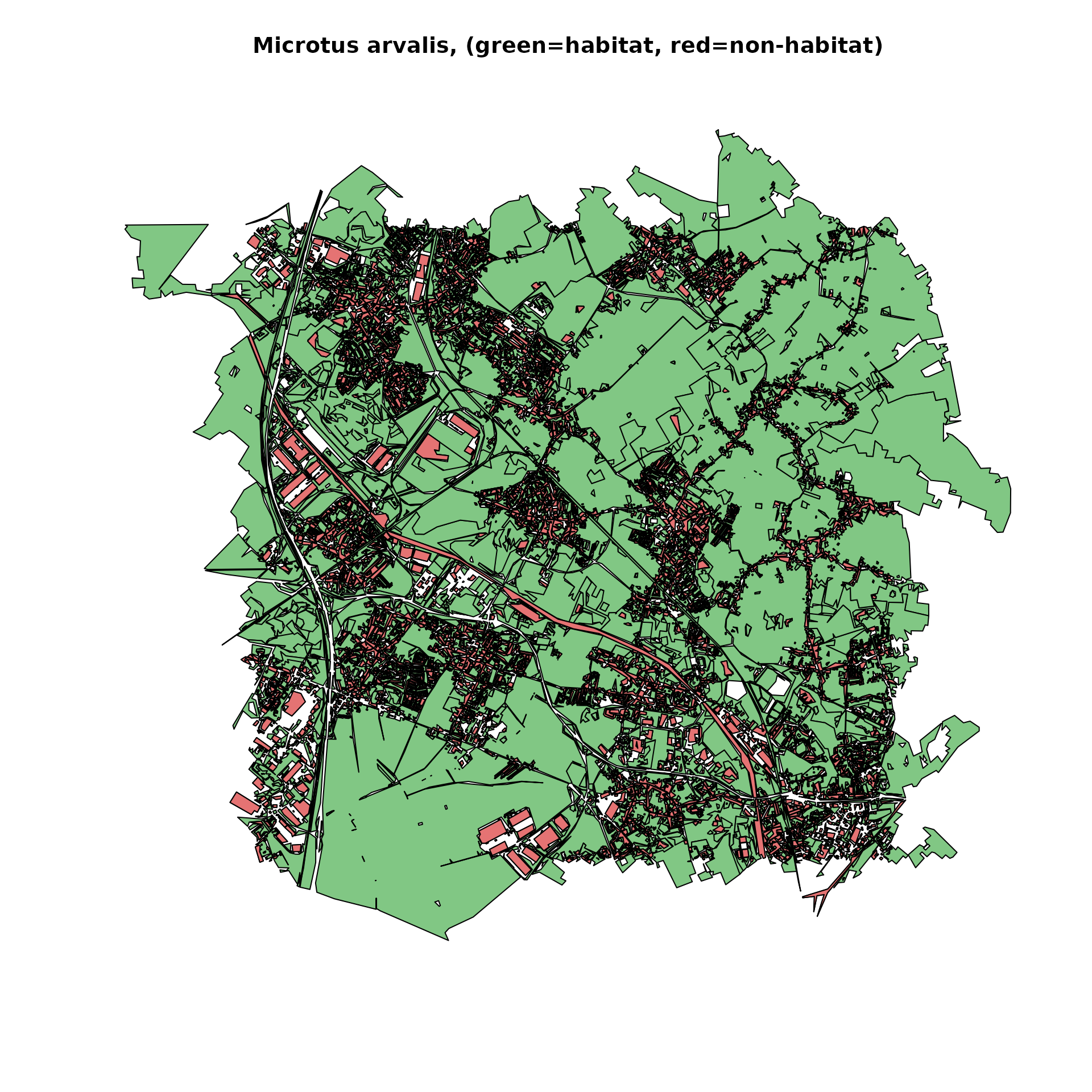

myodes_hab <- join_ocsge_species(ocsge_metaleurop, "Myodes_glareolus")
plot_species_habitat(myodes_hab)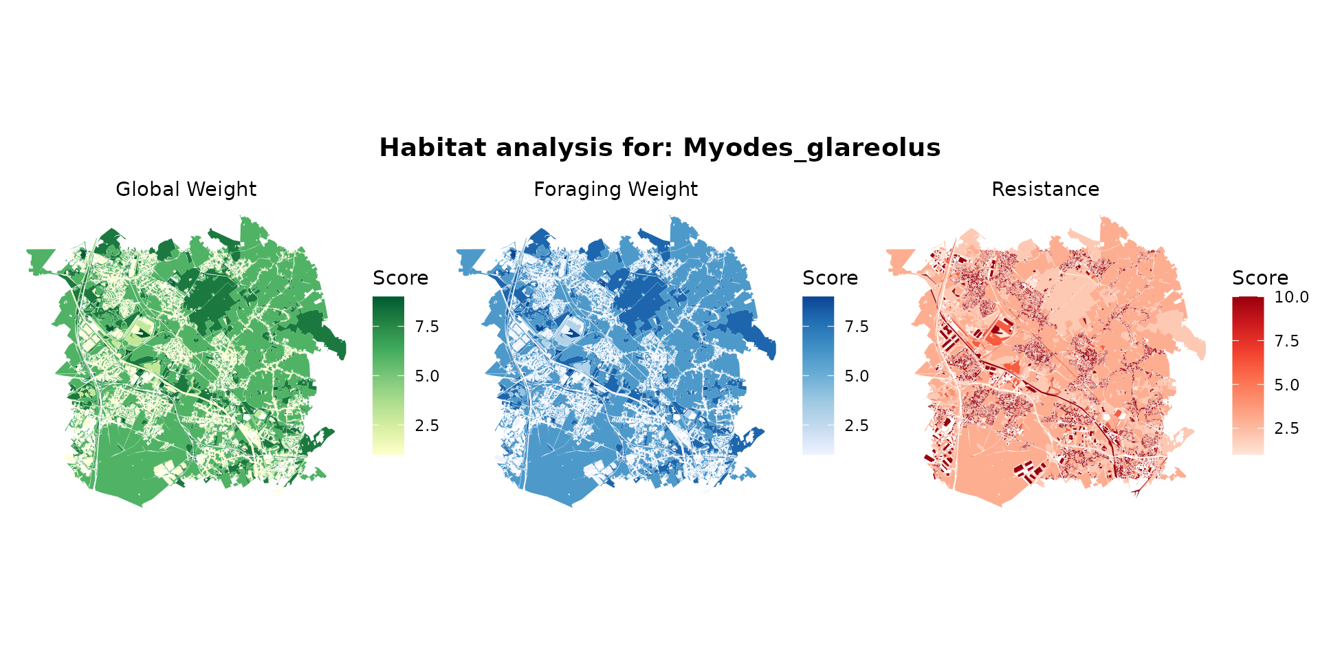

myodes_habitat <- habitat(myodes_hab, habitat=TRUE, weight=myodes_hab$weight_global) |>
  add_nohabitat(myodes_hab[myodes_hab$resistance==10,])

apodemus_hab <- join_ocsge_species(ocsge_metaleurop, "Apodemus_sylvaticus")
plot_species_habitat(apodemus_hab)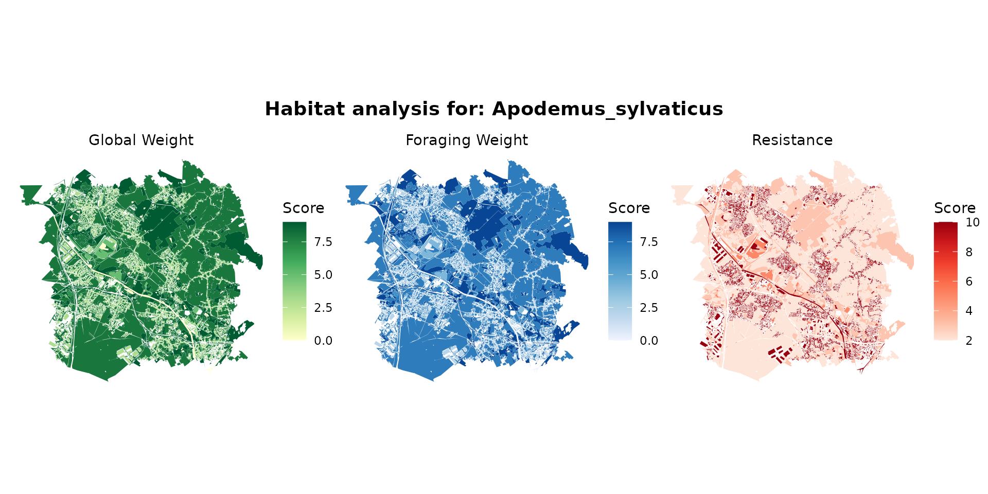

apodemus_habitat <- habitat(apodemus_hab, habitat=TRUE, weight=apodemus_hab$weight_global) |>
  add_nohabitat(apodemus_hab[apodemus_hab$resistance==10,])

sorex_hab <- join_ocsge_species(ocsge_metaleurop, "Sorex_araneus")
plot_species_habitat(sorex_hab)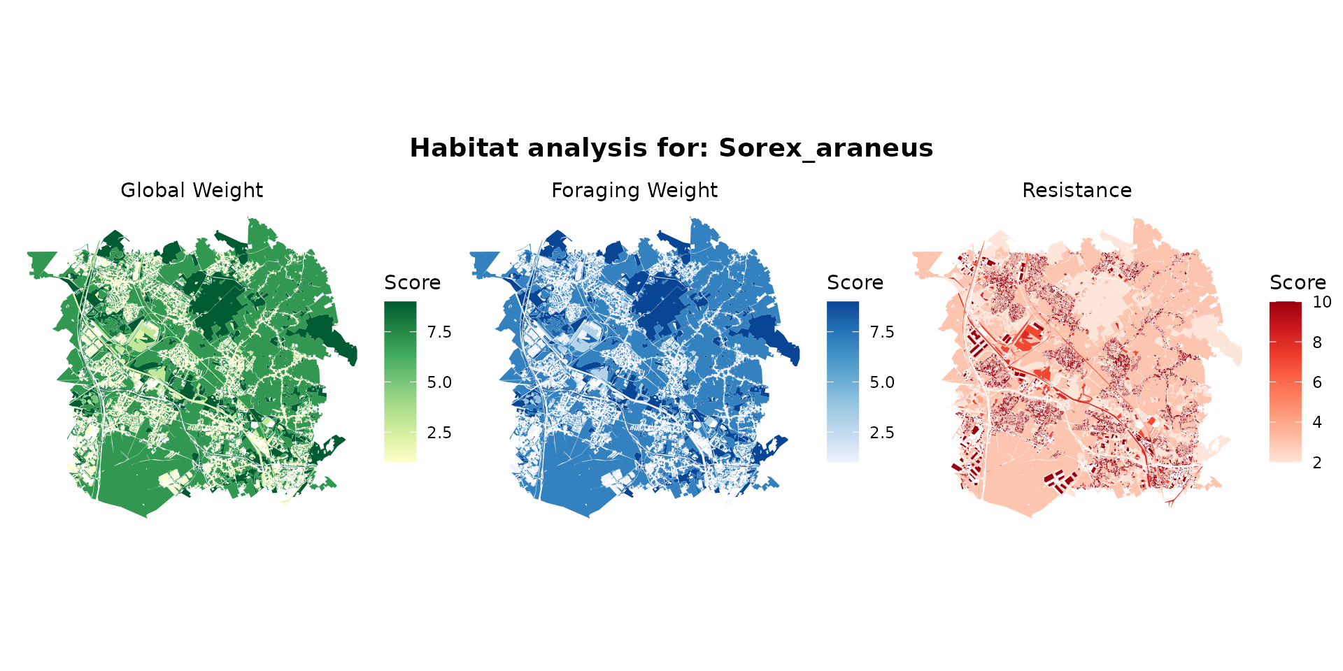

sorex_habitat <- habitat(sorex_hab, habitat=TRUE, weight=sorex_hab$weight_global) |>
  add_nohabitat(sorex_hab[sorex_hab$resistance==10,])

crocidura_hab <- join_ocsge_species(ocsge_metaleurop, "Crocidura_russula")
plot_species_habitat(crocidura_hab)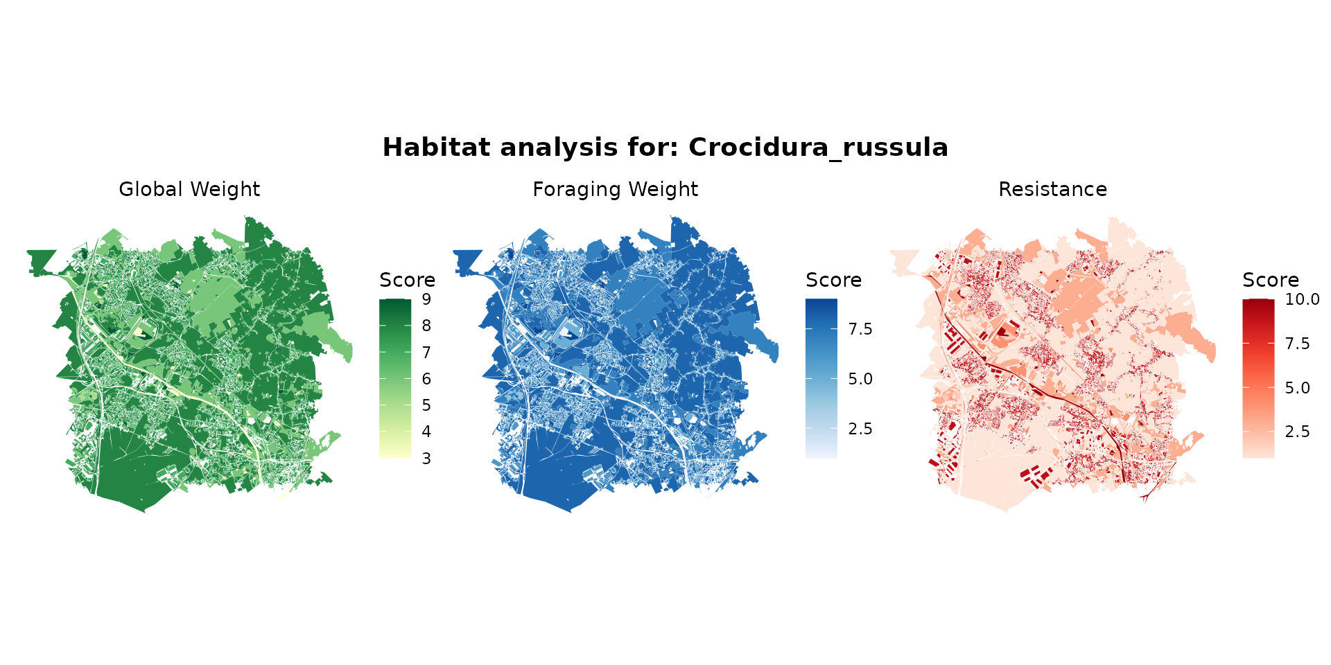

crocidura_habitat <- habitat(sorex_hab, habitat=TRUE, weight=sorex_hab$weight_global) |>
  add_nohabitat(sorex_hab[sorex_hab$resistance==10,])

columba_hab <- join_ocsge_species(ocsge_metaleurop, "Columba_palumbus")
plot_species_habitat(columba_hab)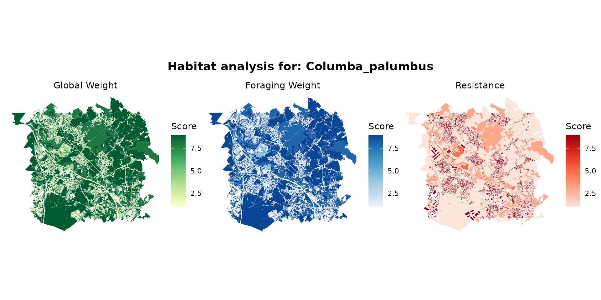

columba_habitat <- habitat(columba_hab, habitat=TRUE, weight=columba_hab$weight_global) |>
  add_nohabitat(columba_hab[columba_hab$resistance==10,])

turdus_hab <- join_ocsge_species(ocsge_metaleurop, "Turdus_merula")
plot_species_habitat(turdus_hab)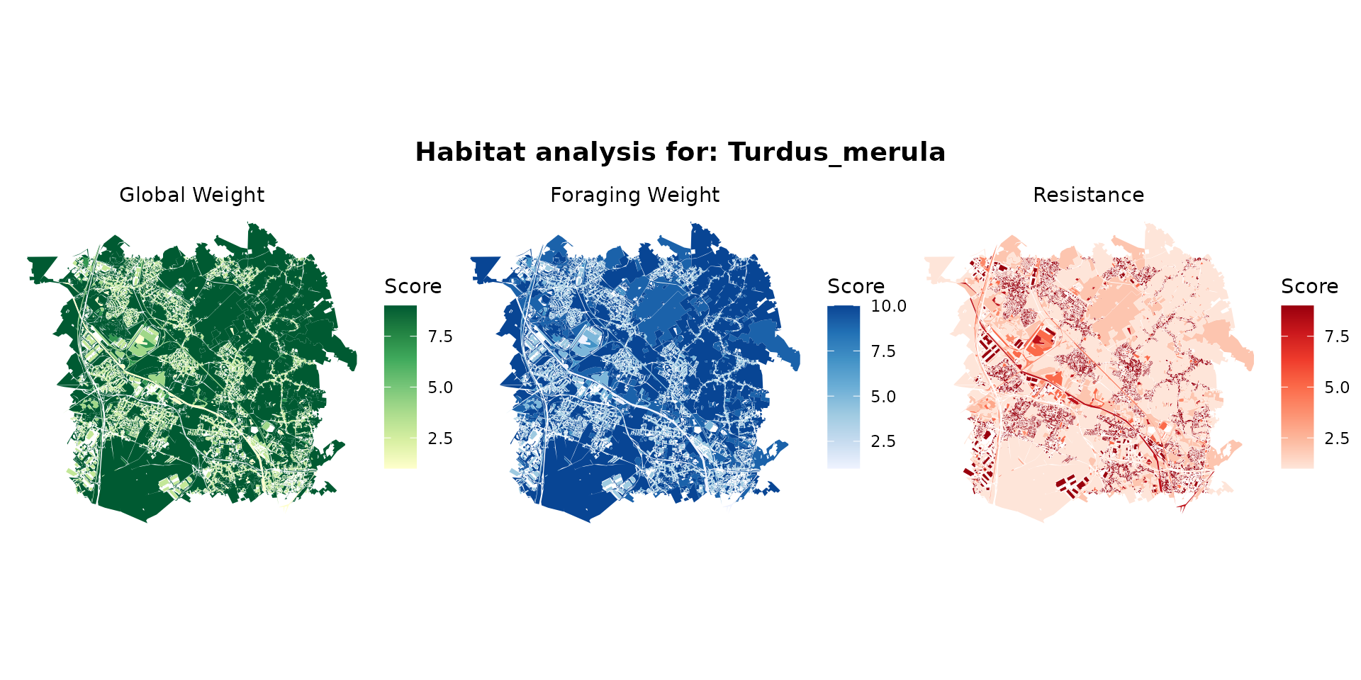

turdus_habitat <- habitat(turdus_hab, habitat=TRUE, weight=turdus_hab$weight_global) |>
  add_nohabitat(turdus_hab[turdus_hab$resistance==10,])

athene_hab <- join_ocsge_species(ocsge_metaleurop, "Athene_noctua")
plot_species_habitat(athene_hab)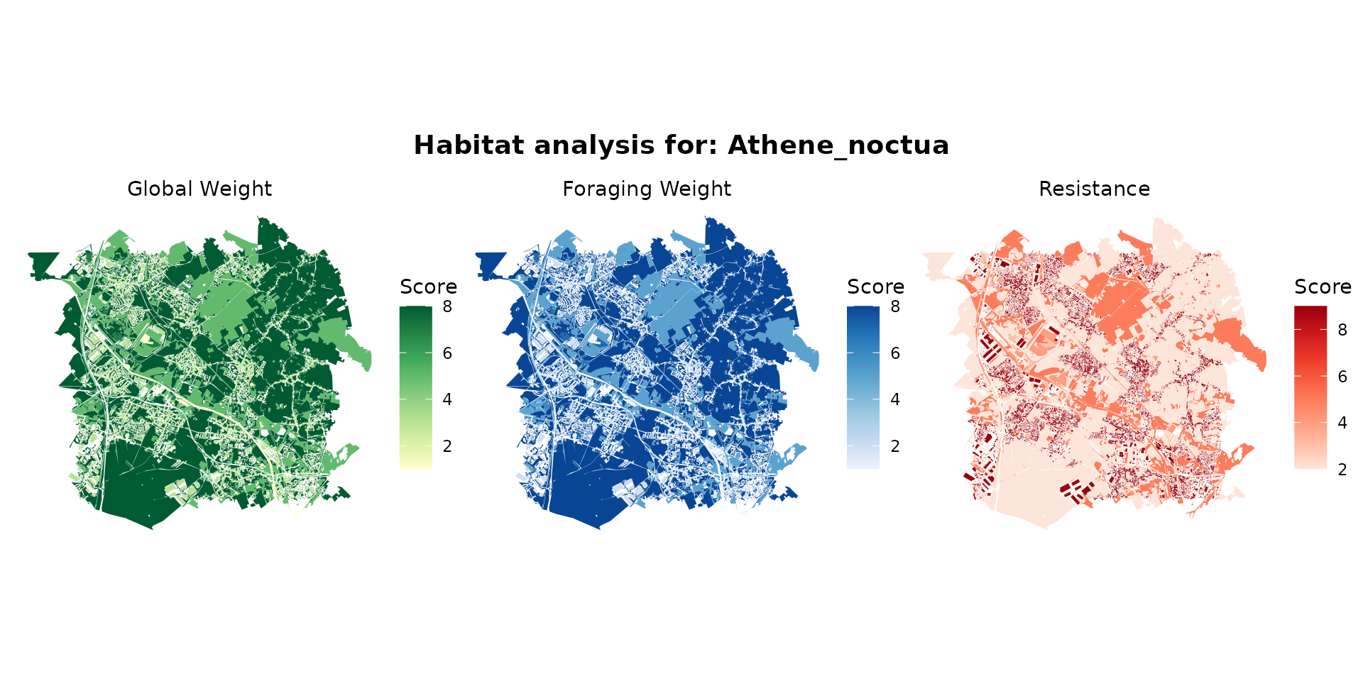

athene_habitat <- habitat(athene_hab, habitat=TRUE, weight=athene_hab$weight_global) |>
  add_nohabitat(athene_hab[athene_hab$resistance==10,])

Rasterize on a same grid frame

At this stage, now that the habitats are defined, we rasterize the habitats based on a default layer, here cd_ground. This allows us to have the same landscape grid so we can successfully overlay all the layers.

# Loading a background concentration raster for a contaminant (Cadmium)
ground_cd <- load_raster_extdata("ground_concentration_cd_compressed.tif")

# We initialize habitat grids (rasters) for each level
rast_soil <- habitat_raster(ground_cd, habitat_soil)
rast_plant <- habitat_raster(ground_cd, habitat_plant)
rast_earthwom <- habitat_raster(ground_cd, habitat_earthworm)
rast_beetle <- habitat_raster(ground_cd, habitat_beetle)

rast_myodes <- habitat_raster(ground_cd, myodes_habitat)
rast_microtus <- habitat_raster(ground_cd, microtus_habitat)
rast_apodemus <- habitat_raster(ground_cd, apodemus_habitat)
rast_crocidura <- habitat_raster(ground_cd, crocidura_habitat)
rast_sorex <- habitat_raster(ground_cd, sorex_habitat)

rast_columba <- habitat_raster(ground_cd, columba_habitat)
rast_turdus <- habitat_raster(ground_cd, turdus_habitat)
rast_athene <- habitat_raster(ground_cd, athene_habitat)

# We create the `raster_stack` of the habitats
stack_habitat <- raster_stack(
  raster_list = list(
    rast_soil, rast_plant, rast_earthwom, rast_beetle,
    rast_myodes, rast_microtus, rast_apodemus, rast_sorex, rast_crocidura,
    rast_columba, rast_turdus, rast_athene),
  names = c("soil", "plant", "earthworm", "beetle",
    "myodes", "microtus", "apodemus", "sorex", "crocidura",
    "columba", "turdus", "athene")
)

Create the spacemodel

spcmdl_berisp_init <- spacemodel(stack_habitat, trophic_df)

plot(spcmdl_berisp_init)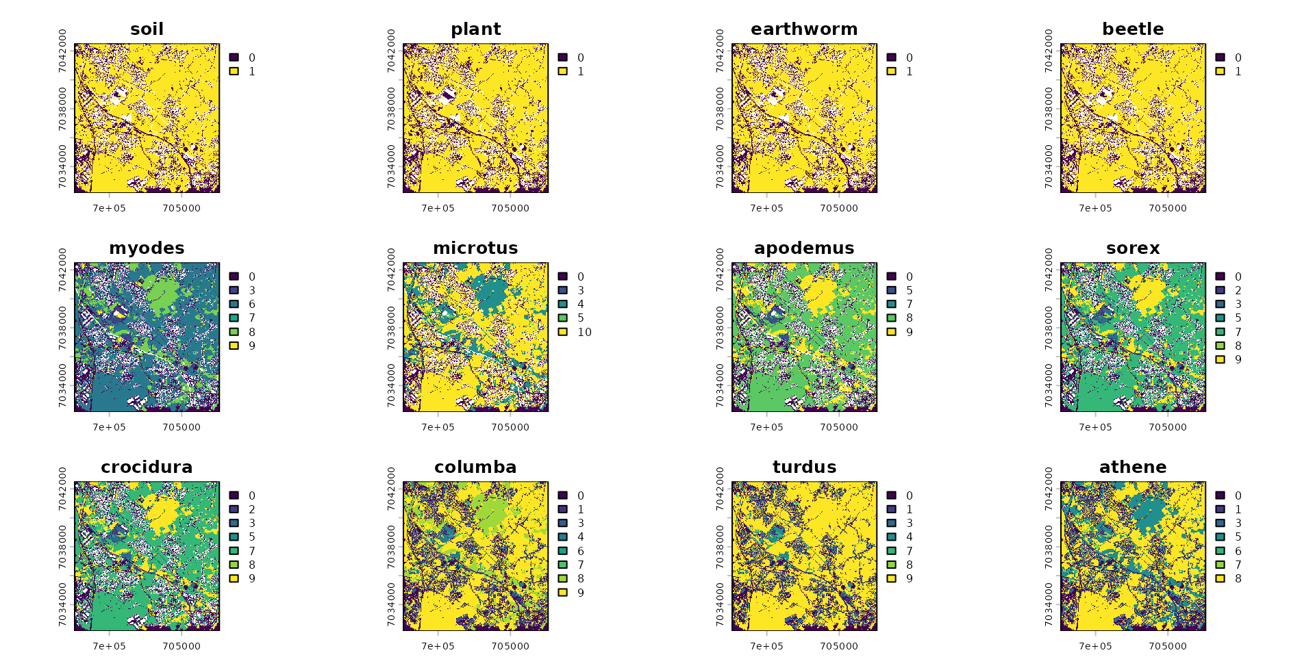

Fluxes

There are several pathways of contamination, which can be divided into two main categories:

Direct contamination: This occurs when an organism absorbs a pollutant directly from its environment. Examples include a fish exposed to waterborne contaminants, an earthworm absorbing pollutants from the soil, or flying arthropods and birds exposed to airborne pollutants. A single organism can also have multiple direct exposure routes; for instance, benthic (sediment-dwelling) invertebrates can be contaminated by both the sediment and the overlying water. To model this, a simple equation is usually sufficient, potentially accounting for environmental properties (e.g., soil pH, organic matter, clay percentage) and species-specific traits (e.g., how a plant might modify the soil-plant interaction).
Trophic contamination: This refers to contamination through dietary intake. To accurately model this route, it is necessary to know the organism’s diet composition (food items consumed), the biomass flux per kilogram of the individual, and the contaminant flux, which is calculated by estimating the contaminant concentration within each specific food resource.

A second challenging aspect for the model is differentiating between exposures (the doses to which organisms are exposed) and accumulated concentrations.

For organisms undergoing direct exposure, there is no need to calculate dietary contamination fluxes. The organism is exposed to 100% of the surrounding medium—and therefore the pollution—and the direct flux equation translates this contamination straight into a body burden.
For trophic contamination, however, it is essential to know the biomass of each specific item in the diet to determine the actual exposure (by multiplying the ingestion rates by the resource concentrations), and finally to calculate the body burdens. These steps can be broken down into separate components, but this is exactly where careful attention is required.

Fluxes: Direct contamination (soil-target transfer for plant and earthworm)

Vegetation

data("bappet_cd")
plt_bappet_cd = bappet_cd[bappet_cd$extraction=="Totale",]

fit_simple_veg_cd <- load_safe("raw_data/fit_simple_veg_cd.rds")
fit_pars <- rstan::extract(fit_simple_veg_cd, c("beta0", "beta1"))
xseq = seq(min(bappet_cd$log10_media_mean), max(bappet_cd$log10_media_mean), length.out=100)
yseq = fit_pars$beta1 %*% t(xseq) + c(fit_pars$beta0)
yseq_q = apply(yseq, 2, quantile, prob = c(0.025, 0.5, 0.975))

# Créer un data.frame pour la ligne
line_data <- data.frame(
  x = xseq,
  y_q50 = yseq_q[2,],
  y_qinf95 = yseq_q[1,],
  y_qsup95 = yseq_q[3,]
)

ggplot() +
  theme_minimal() +
  geom_point(data = plt_bappet_cd,
    aes(x = log10_media_mean, y = log10_plant_mean, color = plant_type)) +
  # geom_line(data = line_data, aes(x = x, y = y_q50), color = "blue", size=1) +
  geom_abline(intercept = -0.488, slope = 0.494, color="red")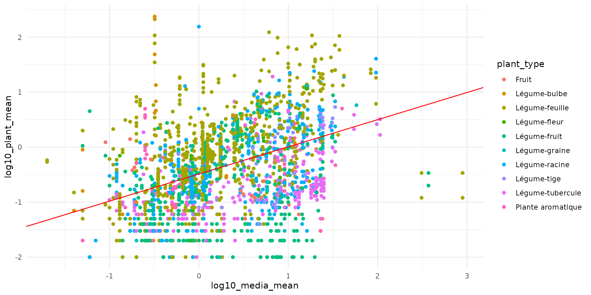

This model give the following equation:

$\log_{10}(C_{vegetation}) = 0.494 * \log_{10}(C_{soil}) -0.488$

For Cadmium, the equation is given in Berisp:

$\log C_{vegetation} = 0.17 + 0.49 \times \log C_{soil} - 0.28 \times \log OM - 0.12 \times pH$

In Eco-SSL, authors use the following equation (Neperian logarithm):

$\ln(C_{vegetation}) = 0.546 * \ln(C_{soil}) - 0.475$

Earthworm

data("earthworm_cd")

fit_simple_worm_cd <- load_safe("raw_data/fit_simple_worm_cd.rds")
fit_pars <- rstan::extract(fit_simple_worm_cd, c("beta0", "beta1"))
xseq = seq(min(earthworm_cd$log10_cd_soil), max(earthworm_cd$log10_cd_soil), length.out=100)
yseq = fit_pars$beta1 %*% t(xseq) + c(fit_pars$beta0)
yseq_q = apply(yseq, 2, quantile, prob = c(0.025, 0.5, 0.975))

# Créer un data.frame pour la ligne
line_data <- data.frame(
  x = xseq,
  y_q50 = yseq_q[2,],
  y_qinf95 = yseq_q[1,],
  y_qsup95 = yseq_q[3,]
)

ggplot() +
  theme_minimal() +
  geom_point(data = earthworm_cd,
    aes(x = log10_cd_soil, y = log10_cd_worm)) +
  # geom_line(data = line_data, aes(x = x, y = y_q50), color = "blue", size=1) +
  geom_abline(intercept = 0.596, slope = 0.983, color="red")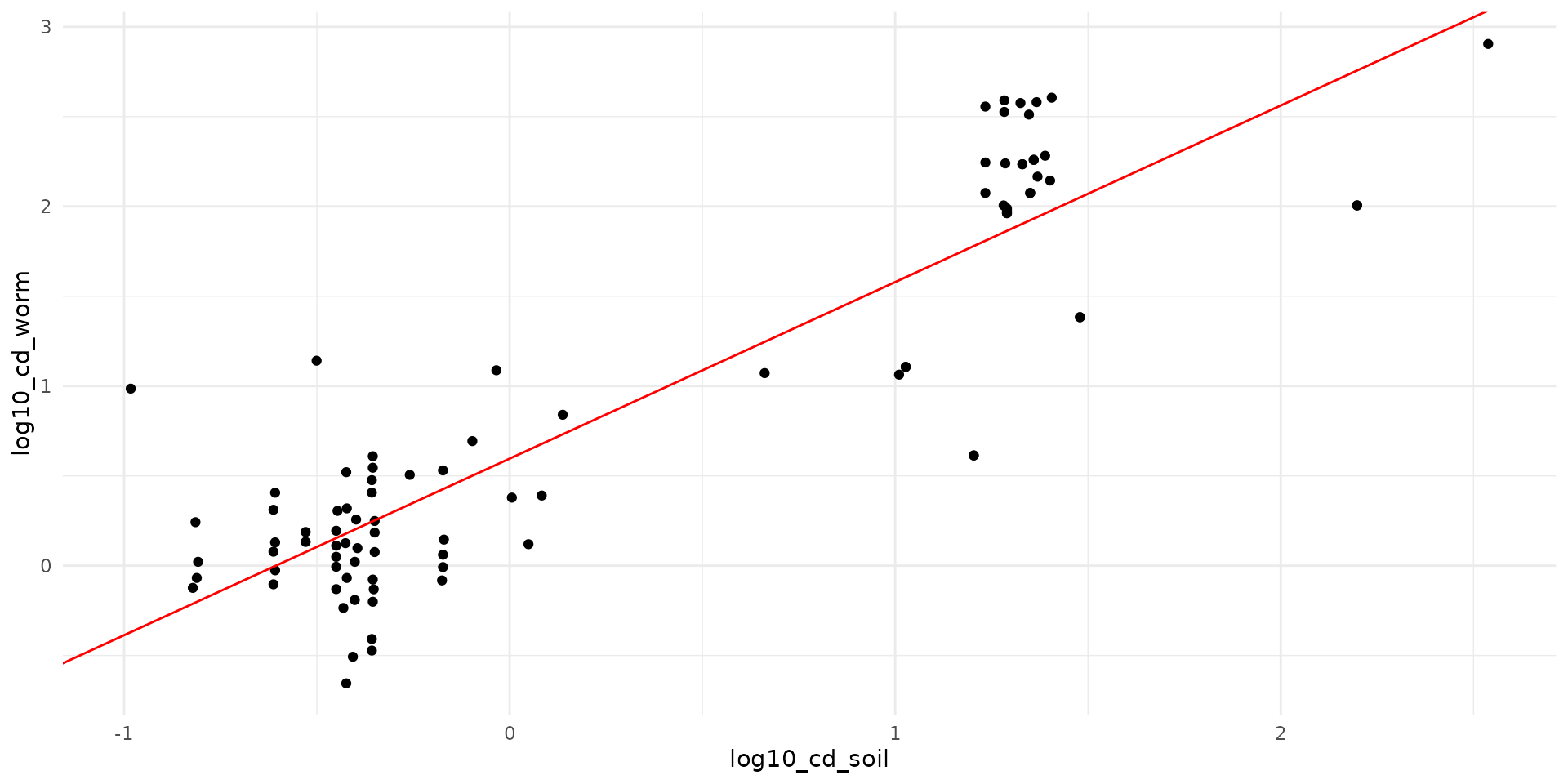

This model give the following equation:

$\log_{10}(C_{earthworm}) = 0.983 * \log_{10}(C_{soil}) + 0.596$

For Cadmium, the equation is given by (Ma et al., 2004):

$\log C_{earthworm} = 2.92 + 0.747 \times \log C_{soil} - 0.5336 \times \log OM - 0.2101 \times pH$

In Eco-SSL, the following equation is given (see Neperian logarithm):

$\ln(C_{earthworm}) = 0.795 * \ln(C_{soil}) + 2.114$

`spacemodel` edit: implementing soil-vegetation and soil-earthworm fluxes

# 1. Assign the actual concentration grid into the "soil" layer
# The Cd in ground layer is in log10(Cd)
spcmdl_berisp_flux <- spcmdl_berisp_init
spcmdl_berisp_flux[["soil"]][] <- ground_cd

# 2. Define the transfer equations (Bioaccumulation / Bioconcentration Factors)
fluxes <- flux(
    spcmdl_berisp_flux,
    default = 1,    # for all other default is 1
    normalize=FALSE # TRUE would weight every link to sum at 1
  ) |>
  add_flux("soil", "plant",  ~ -0.488 + 0.494 * x) |>
  add_flux("soil", "earthworm",  ~ 0.596 + 0.983 * x)

Fluxes: Trophic Contamination (Dietary Exposure)

A little bit of theory

In the Terrasys software, using the framework of the US-EPA, the equation of transfer is given by:

$C_{consumer} = k_{met, consumer} \times BTF_{consumer} \times \frac{FIR_{consumer}}{b_{consumer}} \times \sum_i C_{resource,i} \times p_{i,consumer}$

with:

$p_{i,consumer}$ proportion of that resource $i$ in the diet of the consumer
$BTF_{consumer}$ : the biotransfer factor for the consumer in $day/g$
$FIR_{consumer}$ : the Food Ingestion Rate in $g food / day$ .
$b_{consumer}$ : individual/item biomass of consumer $[g]$ (in average).
$k_{met, consumer}$ : the coefficient of metabolisation. Default is 1.0 is Terrasys.

In the EFSA guidelines for risk assessment on Birds and Mammals, @efsa2023era, the equation of dose of contaminant to which a target is exposed to is given by:

$D_{consumer} = FIR_{consumer} \times \sum_{i} \frac{C_{resource,i}}{b_{consumer}} \times p_{i,consumer} \times PT_{consumer}$

where variable name are already defined except these:

$D_{consumer}$ : dose to which the consumer is exposed to (not yet in body burden),
$PT_{consumer}$ : proportion of the consumer in the area of the contaminated resources (or within the treated area) (spatial overlapping),
$b_{consumer}$ : individual/item biomass of consumer $[g]$ (in average).

The difference between the dose and the internal concentration is gevin in terrasys by:

$k_{met, consumer} \times BTF_{consumer}$

Finally, in the original Berisp documentation, the following equation is used to model the trophic transfer:

$C_{consumer} = \frac{b_{resource}}{b_{consumer}} \times C_{resource} \times \frac{k_{up}}{k_{out}} \left( 1 - \exp^{- c_{out} \times a} \right)$

where:

$b_{resource}$ : average individual/item biomass of resource $[g]$ ,
$b_{consumer}$ : average individual/item biomass of consumer $[g]$ ,
$C_{resource}$ : concentration of substance in resource (e.g. $ppm=[ug.g^{-1}]=[mg.kg^{-1}]$ ),
$C_{resource}$ : concentration of substance in resource (e.g. $ppm=[ug.g^{-1}]=[mg.kg^{-1}]$ ),
$k_{up}$ : assimilation efficiency of food $[n.d.]$ ,
$k_{out}$ : excretion rate of food, $[day^{-1}]$
$a$ : average age of the consumer $[day]$ ,

We can see that $b_{resource}$ is the value given by $FIR_{consumer} \times p_{i,consumer}$ in previous equations used in Terrasys software or by the EFSA.

Further assumptions:

We could reduce complexity by assuming a single $BF_{resource, consumer} = k_{up}/k_{out}$ paramater since parameterisation of $k_{up}$ and $k_{out}$ are not identifiable in this equation. The idea is to re-use the $BF_{resource, consumer} = k_{met} BTF_{consumer} $ from the Terrasys model. .
We can also assume that individuals are old enough to reach a stability of contamination, so as: $C_{consumer} = \frac{b_{resource}}{b_{consumer}} \times C_{resource} \times BF_{resource, consumer}$
the $b_{resource}$ is the Food Ingestion Rate of the consumer ( $[g food / g consumer / day]$ ) times the proportion of that resource in the diet ( $p_{resource, consumer}$ ).

With this assumption, the equation is:

$C_{consumer} = \frac{FIR_{consumer}}{b_{consumer}} \times \sum_i p_{i, consumer} \times C_{i} \times BF_{i, consumer}$

Fluxes of Biomass FIRbw

`spacemodel` edit: implementing fluxes of biomass

Fluxes of Contaminants

Carabid

In Berisp, authors use the following direct soil-target equation:

$\log(C_{carabid}) = -1 + 0.6 * \log(C_{soil})$

In our model, ground beetles eats plants and earthworm. So we are going to use a transfer model.

In Terrasys software, the equation for the BTF was given by:

$\log_{10}(BTF_{soil_invertebrates}) = 1.588 - 0.578 \times \log_{10}(k_{ow})$

with:

$BTF_i$ : biotransfer factor
$k_{ow}$ : octanol /water partition coefficient.

But the problem is that $1.588 - 0.578 * (-1.65))=$ would give a $BTF$ of

$C_{\text{terrestrial invertebrates}} = BTF_veg_inv × C_vegetation$

Mammals

In Terrasys software, the equation for the BTF from the US-EPA (1999c) was:

$\log_{10}(BTF_{mammal}) = -7.6 + \log_{10}(k_{ow})$

Birds

In Terrasys software, the equation for the BTF from the US-EPA (1999c) was:

$BTF_{bird} = 0.8 BTF_{mammal} = 0.8 \times \left( 10^{-7.6 + \log_{10}(k_{ow})}\right)$

`spacemodel` edit: implementing fluxes of contaminant

Important: After this step: concentration in soil, plant and earthworm are log10 scaled ppm, while concentration in beetle, mammal and birds are in ppm.

BTF_beetle <- 0.1   
BTF_mammal_herb <- 0.05
BTF_mammal_ins <- 0.025 # 0.08
BTF_bird   <- 0.04  # (0.8 * 0.05)
species_traits <- species_traits %>%
  mutate(
    BTF = case_when(
      species == "beetle" ~ BTF_beetle,
      species %in% c("myodes", "microtus") ~ BTF_mammal_herb,
      species %in% c("apodemus", "sorex", "crocidura") ~ BTF_mammal_ins,
      species %in% c("columba", "turdus", "athene") ~ BTF_bird
    )
  )
vec_BTF <- setNames(species_traits$BTF, species_traits$species)

# Définition des transferts de flux dans le spacemodel
fluxes <- flux(
    spcmdl_berisp_flux, 
    default = 1,
    normalize = FALSE
  ) |>
  # 1. Contamination directe (les équations donnent le log10 de la concentration)
  add_flux("soil", "plant",  ~ -0.488 + 0.494 * x) |>
  add_flux("soil", "earthworm",  ~ 0.596 + 0.983 * x) |>
  # 2. Invertébrés (beetle)
  add_flux("soil", "beetle", ~ 10^x * vec_FIRbw["beetle"] * vec_BTF["beetle"]) |>
  add_flux("plant", "beetle", ~ 10^x * vec_FIRbw["beetle"] * vec_BTF["beetle"]) |>
  add_flux("earthworm", "beetle", ~ 10^x * vec_FIRbw["beetle"] * vec_BTF["beetle"]) |>
  # 3. Mammifères - Myodes (Bank vole)
  add_flux("soil", "myodes", ~ 10^x * vec_FIRbw["myodes"] * vec_BTF["myodes"]) |>
  add_flux("plant", "myodes", ~ 10^x * vec_FIRbw["myodes"] * vec_BTF["myodes"]) |>
  add_flux("earthworm", "myodes", ~ 10^x * vec_FIRbw["myodes"] * vec_BTF["myodes"]) |>
  add_flux("beetle", "myodes", ~ x * vec_FIRbw["myodes"] * vec_BTF["myodes"]) |>
  # 4. Mammifères - Microtus (Common vole)
  add_flux("soil", "microtus", ~ 10^x * vec_FIRbw["microtus"] * vec_BTF["microtus"]) |>
  add_flux("plant", "microtus", ~ 10^x * vec_FIRbw["microtus"] * vec_BTF["microtus"]) |>
  # 5. Mammifères - Apodemus (Wood mouse)
  add_flux("soil", "apodemus", ~ 10^x * vec_FIRbw["apodemus"] * vec_BTF["apodemus"]) |>
  add_flux("plant", "apodemus", ~ 10^x * vec_FIRbw["apodemus"] * vec_BTF["apodemus"]) |>
  add_flux("earthworm", "apodemus", ~ 10^x * vec_FIRbw["apodemus"] * vec_BTF["apodemus"]) |>
  add_flux("beetle", "apodemus", ~ x * vec_FIRbw["apodemus"] * vec_BTF["apodemus"]) |>
  # 6. Mammifères - Musaraignes (Sorex & Crocidura)
  add_flux("soil", "sorex", ~ 10^x * vec_FIRbw["sorex"] * vec_BTF["sorex"]) |>
  add_flux("earthworm", "sorex", ~ 10^x * vec_FIRbw["sorex"] * vec_BTF["sorex"]) |>
  add_flux("beetle", "sorex", ~ x * vec_FIRbw["sorex"] * vec_BTF["sorex"]) |>
  add_flux("soil", "crocidura", ~ 10^x * vec_FIRbw["crocidura"] * vec_BTF["crocidura"]) |>
  add_flux("earthworm", "crocidura", ~ 10^x * vec_FIRbw["crocidura"] * vec_BTF["crocidura"]) |>
  add_flux("beetle", "crocidura", ~ x * vec_FIRbw["crocidura"] * vec_BTF["crocidura"]) |>
  # 7. Oiseaux - Pigeon (Columba)
  add_flux("plant", "columba", ~ 10^x * vec_FIRbw["columba"] * vec_BTF["columba"]) |>
  # 8. Oiseaux - Merle noir (Turdus)
  add_flux("plant", "turdus", ~ 10^x * vec_FIRbw["turdus"] * vec_BTF["turdus"]) |>
  add_flux("earthworm", "turdus", ~ 10^x * vec_FIRbw["turdus"] * vec_BTF["turdus"]) |>
  add_flux("beetle", "turdus", ~ x * vec_FIRbw["turdus"] * vec_BTF["turdus"]) |>
  # 9. Oiseaux - Chouette chevêche (Athene) - Super prédateur
  add_flux("earthworm", "athene", ~ 10^x * vec_FIRbw["athene"] * vec_BTF["athene"]) |>
  add_flux("beetle", "athene", ~ x * vec_FIRbw["athene"] * vec_BTF["athene"]) |>
  add_flux("myodes", "athene", ~ x * vec_FIRbw["athene"] * vec_BTF["athene"]) |>
  add_flux("microtus", "athene", ~ x * vec_FIRbw["athene"] * vec_BTF["athene"]) |>
  add_flux("apodemus", "athene", ~ x * vec_FIRbw["athene"] * vec_BTF["athene"]) |>
  add_flux("sorex", "athene", ~ x * vec_FIRbw["athene"] * vec_BTF["athene"]) |>
  add_flux("crocidura", "athene", ~ x * vec_FIRbw["athene"] * vec_BTF["athene"])

Movement of population (extended habitat) dispersion in landscape

# Calcul des noyaux de dispersion en fonction de l'écologie spatiale (rayons de mobilité)
# Invertébrés terrestres
k_beetle    <- compute_kernel(radius=10, GSD=25, size_std=0.5)

# Micromammifères (Rongeurs et Insectivores)
k_sorex     <- compute_kernel(radius=25, GSD=25, size_std=0.05)
k_crocidura <- compute_kernel(radius=25, GSD=25, size_std=0.05)
k_microtus  <- compute_kernel(radius=30, GSD=25, size_std=0.05)
k_myodes    <- compute_kernel(radius=40, GSD=25, size_std=0.05)
k_apodemus  <- compute_kernel(radius=60, GSD=25, size_std=0.05)

# Oiseaux
k_turdus    <- compute_kernel(radius=150, GSD=25, size_std=0.05)
k_columba   <- compute_kernel(radius=300, GSD=25, size_std=0.05)
k_athene    <- compute_kernel(radius=800, GSD=25, size_std=0.01)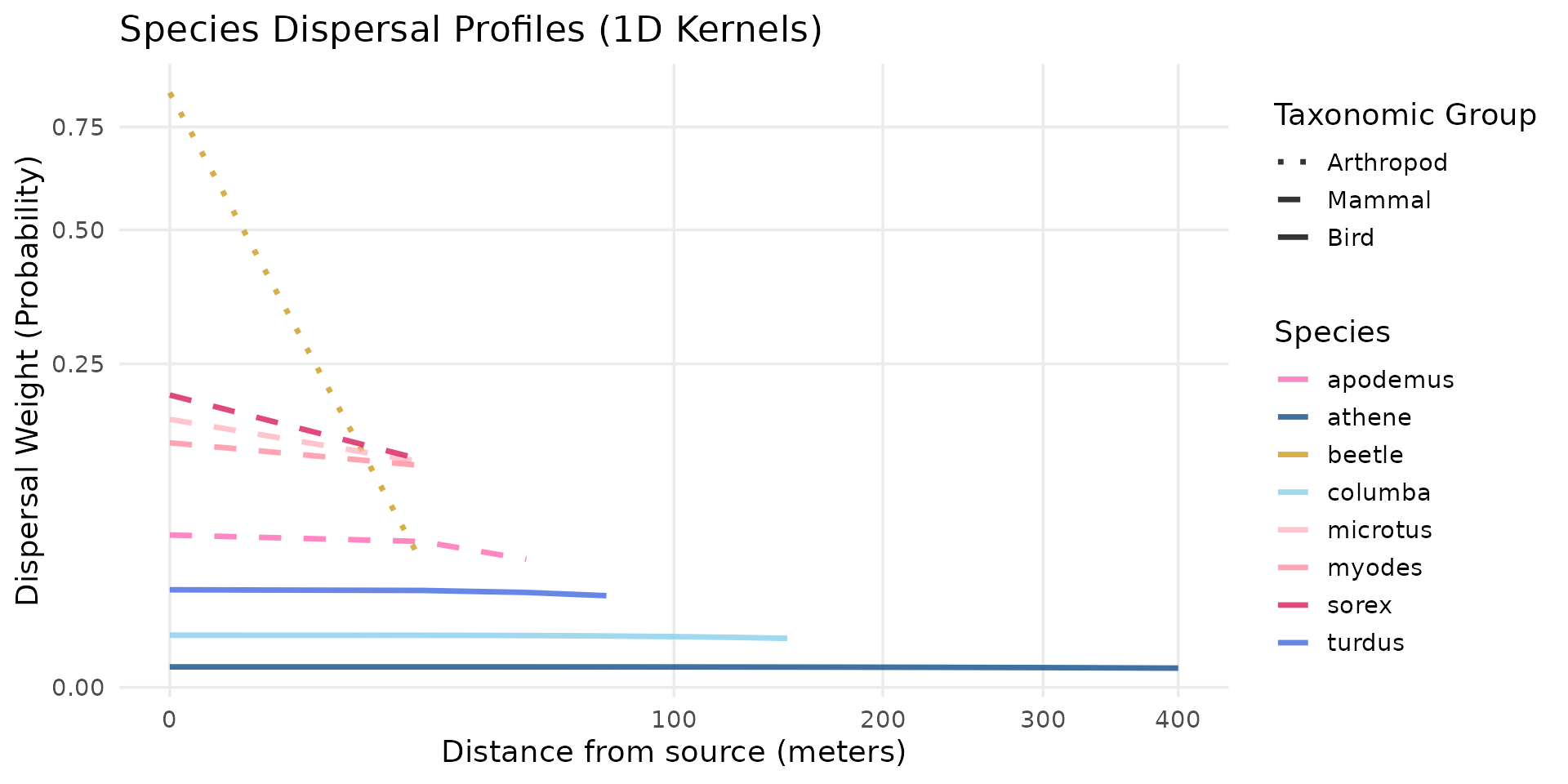

Representation of kernels

Compute dispersal

# Application de la dispersion sur l'objet spacemodel (avec les flux calculés précédemment)
spcmdl_dispersal_init <- spcmdl_berisp_init |>
  dispersal("beetle",    method="convolution", method_option=list(kernel=k_beetle)) |>
  dispersal("sorex",     method="convolution", method_option=list(kernel=k_sorex)) |>
  dispersal("crocidura", method="convolution", method_option=list(kernel=k_crocidura)) |>
  dispersal("microtus",  method="convolution", method_option=list(kernel=k_microtus)) |>
  dispersal("myodes",    method="convolution", method_option=list(kernel=k_myodes)) |>
  dispersal("apodemus",  method="convolution", method_option=list(kernel=k_apodemus)) |>
  dispersal("turdus",    method="convolution", method_option=list(kernel=k_turdus)) |>
  dispersal("columba",   method="convolution", method_option=list(kernel=k_columba)) |>
  dispersal("athene",    method="convolution", method_option=list(kernel=k_athene))

plot(spcmdl_dispersal_init)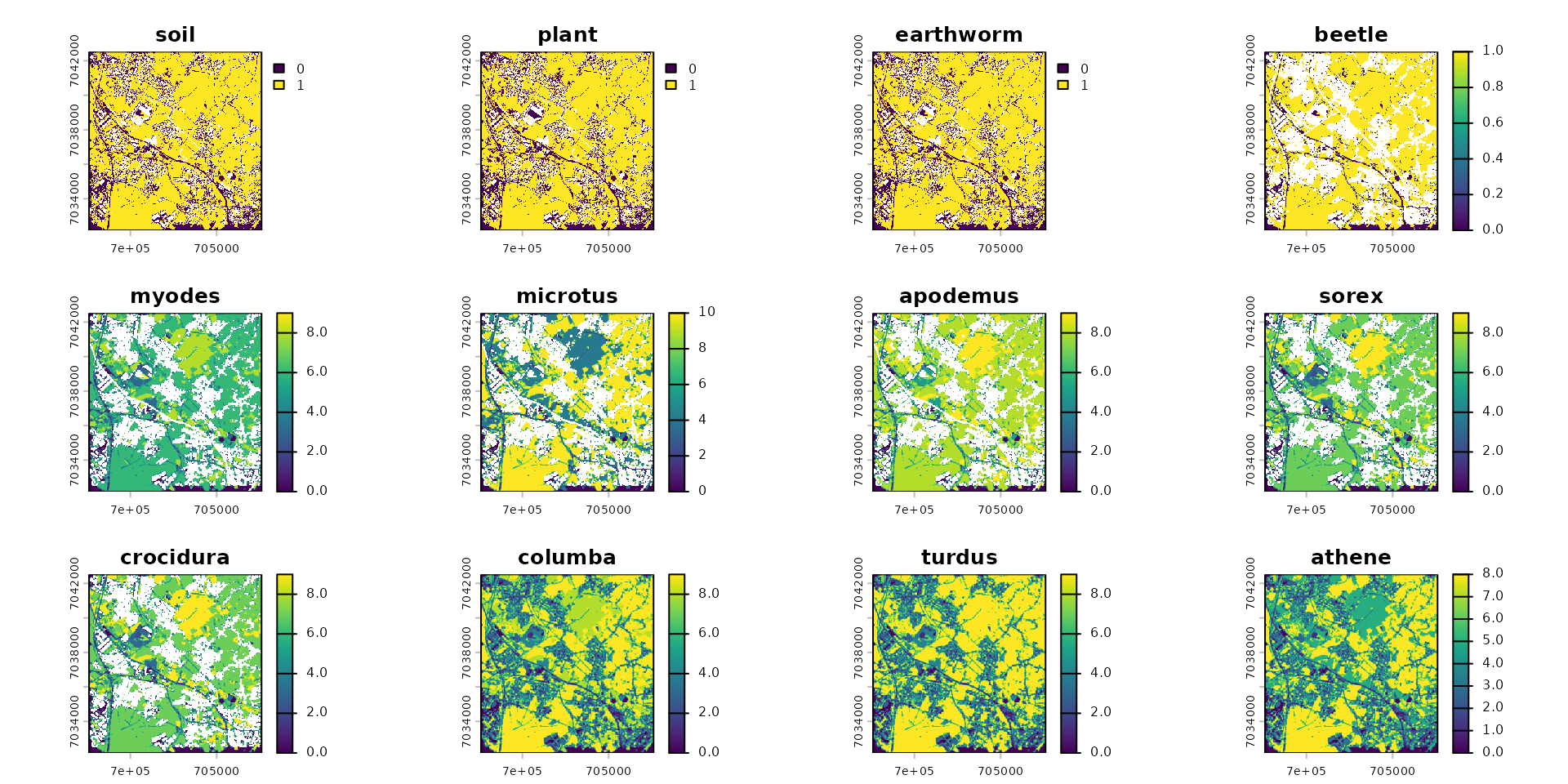

That we can normalized:

species_to_scale <- c("myodes", "microtus", "apodemus", "sorex", "crocidura", 
                      "columba", "turdus", "athene")
spcmdl_dispersal_init[[species_to_scale]] <- spcmdl_dispersal_init[[species_to_scale]] / 10
plot(spcmdl_dispersal_init)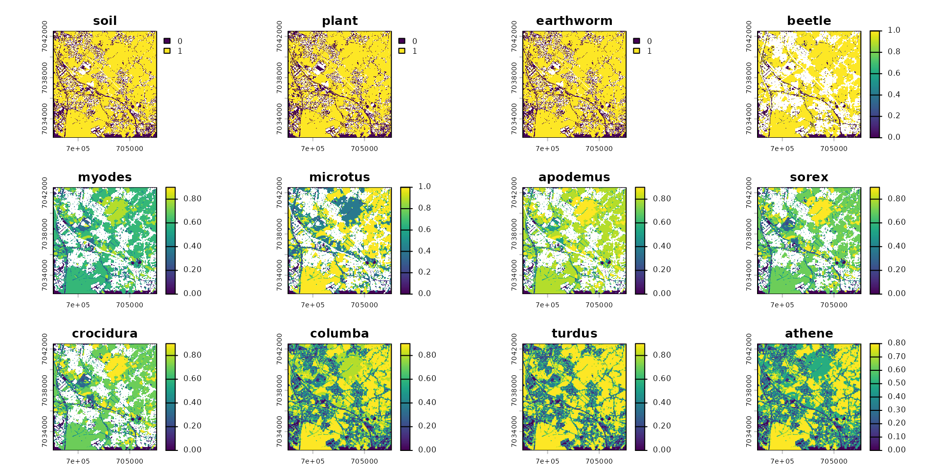

# Application de la dispersion sur l'objet spacemodel (avec les flux calculés précédemment)
spcmdl_dispersal_flux <- spcmdl_berisp_flux |>
  dispersal("beetle",    method="convolution", method_option=list(kernel=k_beetle)) |>
  dispersal("sorex",     method="convolution", method_option=list(kernel=k_sorex)) |>
  dispersal("crocidura", method="convolution", method_option=list(kernel=k_crocidura)) |>
  dispersal("microtus",  method="convolution", method_option=list(kernel=k_microtus)) |>
  dispersal("myodes",    method="convolution", method_option=list(kernel=k_myodes)) |>
  dispersal("apodemus",  method="convolution", method_option=list(kernel=k_apodemus)) |>
  dispersal("turdus",    method="convolution", method_option=list(kernel=k_turdus)) |>
  dispersal("columba",   method="convolution", method_option=list(kernel=k_columba)) |>
  dispersal("athene",    method="convolution", method_option=list(kernel=k_athene))

plot(spcmdl_dispersal_flux)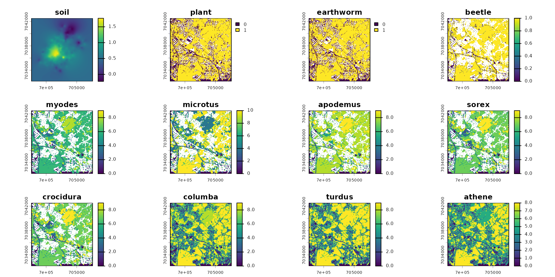

Transfer of food and contaminant

To extract both the exposure (ingested dose) and the impregnation (body burden) without running the model twice, we can use a simple mathematical trick. Because our trophic network must propagate the body burden from prey to predator, the spatial model calculates the final tissue concentrations by default. However, since the transfer equation for all our animals is strictly linear—where Body Burden = Exposure × BTF—we can easily retrieve the initial exposure post-simulation using the inverse operation: Exposure = Body Burden / BTF. Here is how to implement this cleanly in R to extract both metrics from your final spatial model:

Kernel of foraging

In spatial trophic modeling, it is crucial to distinguish between a species’ habitat distribution (where it lives) and its foraging range (where it eats).

The foraging_kernels list provided to the transfer() function specifically defines this foraging range: it allows the model to scan the surrounding pixels and average the contamination of the ingested prey.

However, because the habitat maps were already smoothed during the initial dispersal() step, we must carefully select the exposure_weighting method to avoid a mathematical error known as double smoothing (applying the kernel twice to the habitat):

Avoid “diffuse”: This would apply the spatial kernel a second time to the habitat map, artificially expanding the species’ presence.
Use “potential”: This maps the pure environmental risk by calculating the theoretical exposure an animal would face if placed on any given pixel, regardless of its actual habitat probability.
Use “local”: This calculates the realized ecological risk by weighting the exposure strictly by the pre-dispersed habitat probability already calculated in the previous step.

foraging_kernels <- list(
  beetle    = k_beetle,
  sorex     = k_sorex,
  crocidura = k_crocidura,
  microtus  = k_microtus,
  myodes    = k_myodes,
  apodemus  = k_apodemus,
  turdus    = k_turdus,
  columba   = k_columba,
  athene    = k_athene
)

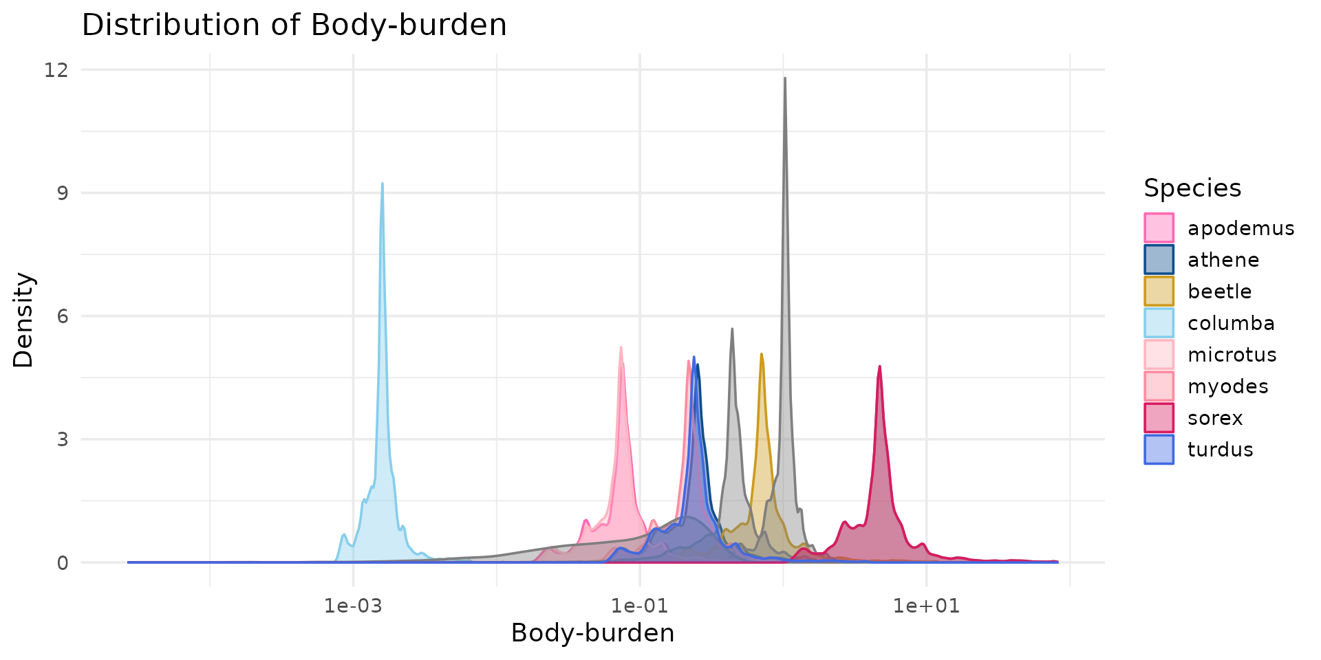
Body-Burden: compute impregnation

# Calculate the final exposure/body burden for all species in the food web
spcmdl_impregnation <- transfer(
  # spacemodel = spcmdl_dispersal_flux,
  spacemodel = spcmdl_berisp_flux,
  kernels    = foraging_kernels,
  fluxes     = fluxes,
  # exposure_weighting = "local"
  exposure_weighting = "potential"
  # exposure_weighting = "diffuse"
)
plot(spcmdl_impregnation)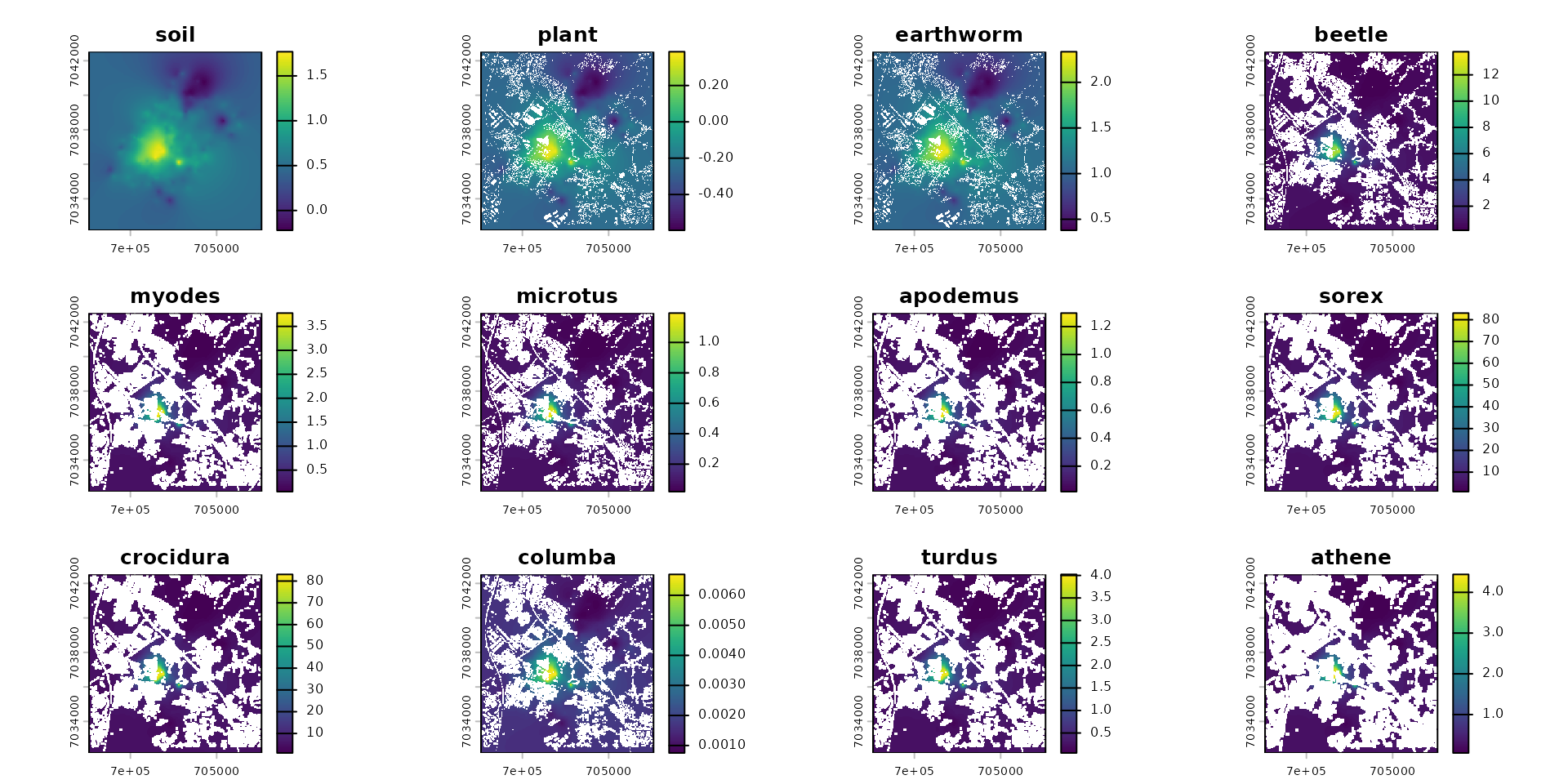

Exposure Extract exposure

# Extraire TOUTES les couches du SpatRaster dans un seul data.frame
df_all <- as.data.frame(spcmdl_impregnation, na.rm = TRUE)

# Transformer le tableau "large" (1 colonne = 1 espèce) 
# en format "long" (1 ligne = 1 observation d'une espèce)
df_long <- pivot_longer(
  df_all,
  cols = everything(),
  names_to = "species",
  values_to = "concentration"
)

# Créer le graphique de densité globale
ggplot(df_long, aes(x = concentration, fill = species, color = species)) +
  geom_density(alpha = 0.4) + 
  scale_fill_manual(values = species_colors) +
  scale_color_manual(values = species_colors) +
  theme_minimal(base_size = 14) +
  scale_x_log10() +
  labs(
    title = "Distribution of Body-burden",
    x = "Body-burden",
    y = "Density",
    fill = "Species",
    color = "Species"
  ) +
  theme(
    legend.position = "right"
  )

species_names <- species_traits$species
spcmdl_exposure <- spcmdl_impregnation
spcmdl_exposure[[species_names]] <- spcmdl_exposure[[species_names]] / vec_BTF
spcmdl_diet_conc <- spcmdl_exposure
spcmdl_diet_conc[[species_names]] <- spcmdl_diet_conc[[species_names]] / vec_FIRbw

Absolute value mg/g per individual

# absolute value mg/g per individual
plot(spcmdl_exposure)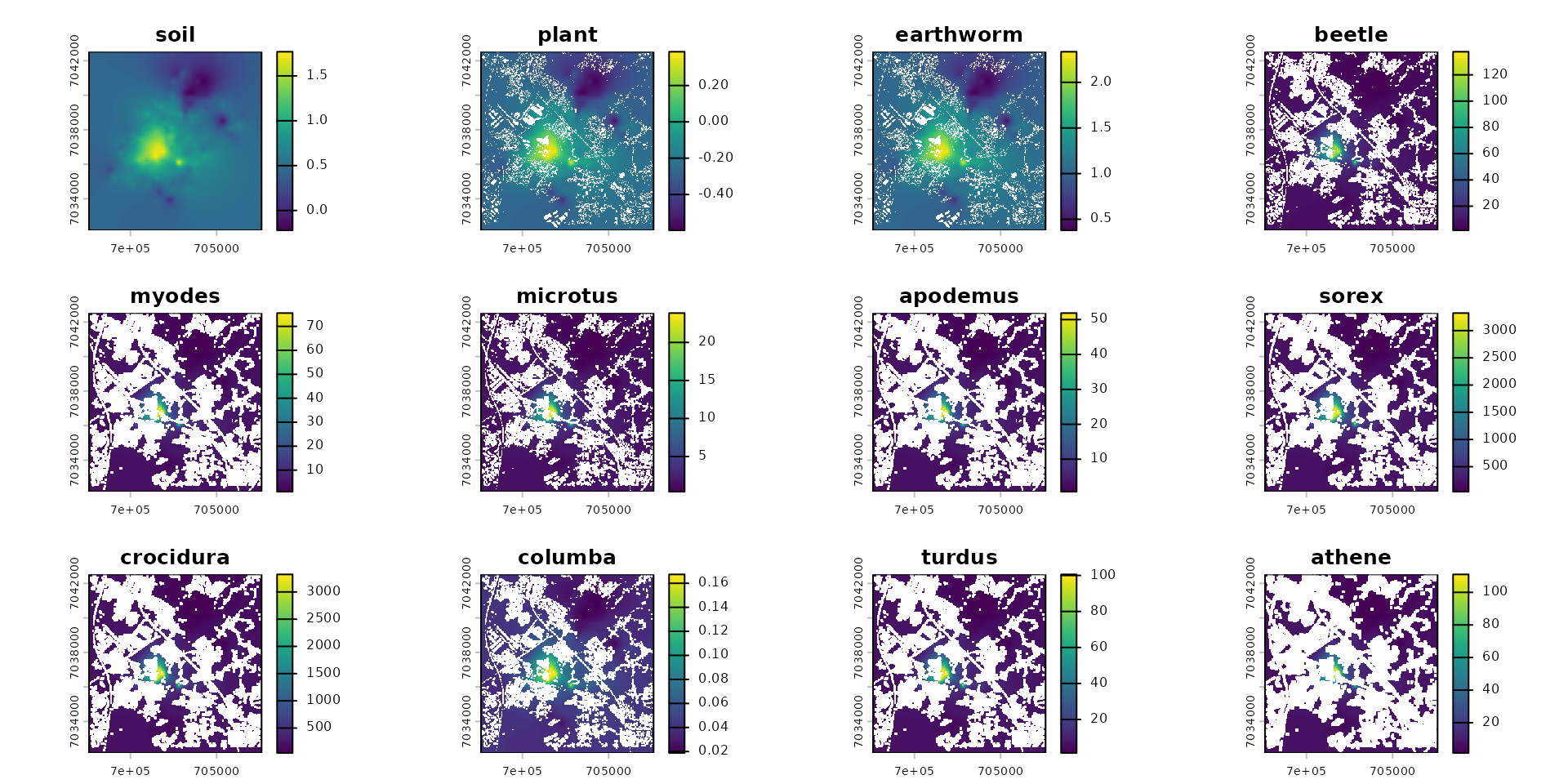

Relative value as daily dose in mg/g/kg bw

# absolute value mg/g/kg bw
plot(spcmdl_diet_conc)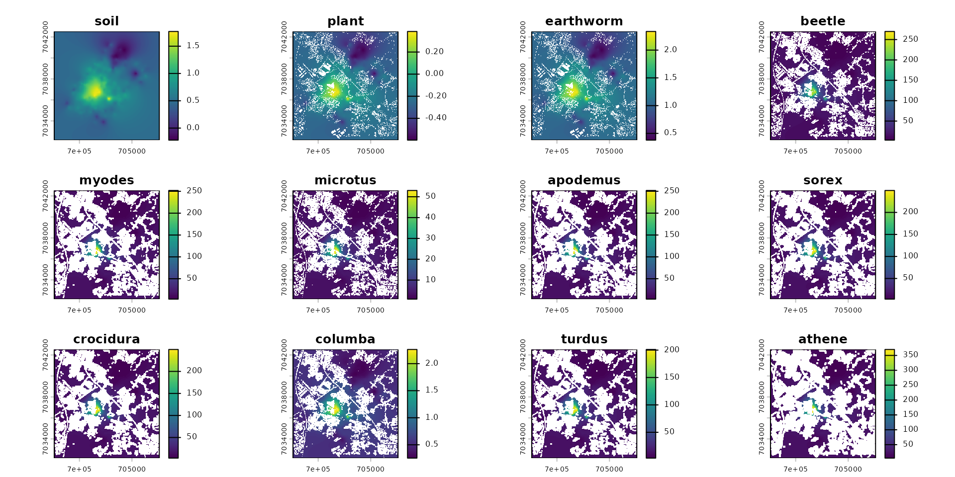

Compared to data

Plants

Earthworm

data("earthworm_cd")

ggplot() +
  theme_minimal() +
  geom_point(data=earthworm_cd, aes(x=log10_cd_soil, y=log10_cd_worm)) +
  geom_point(data=df_all, aes(x=soil, y=earthworm), col="red")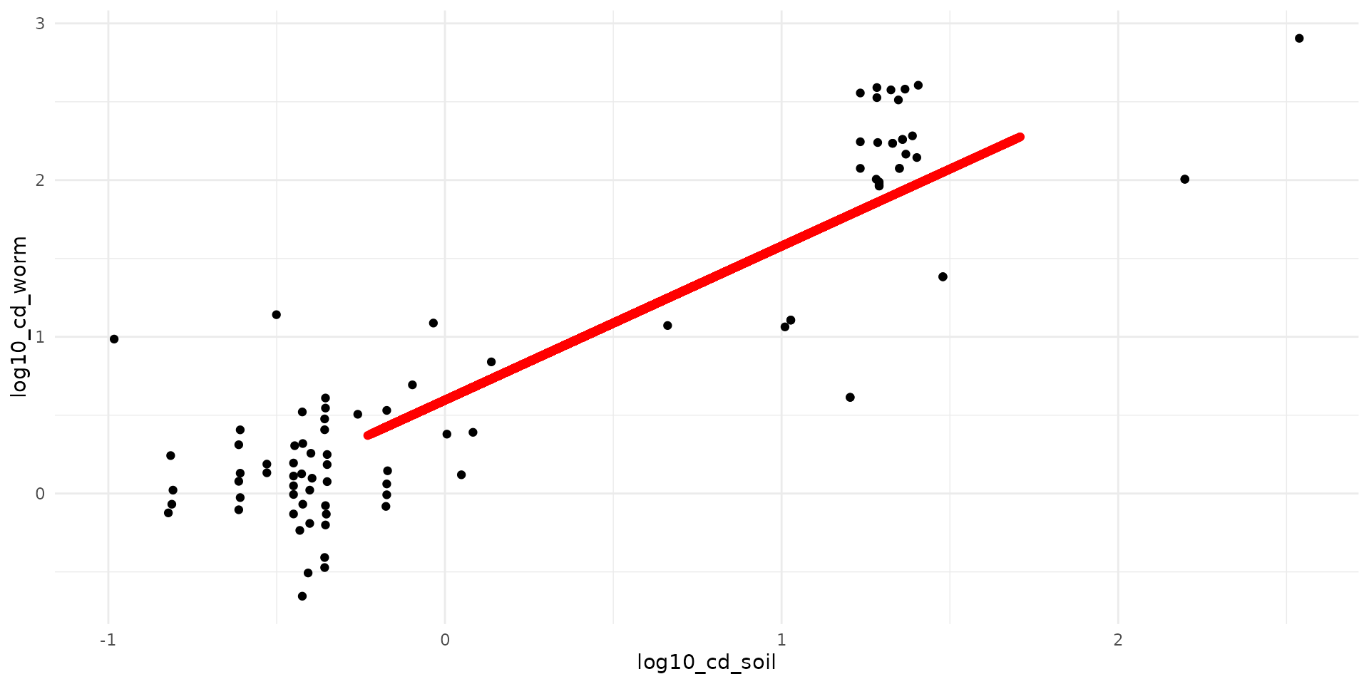

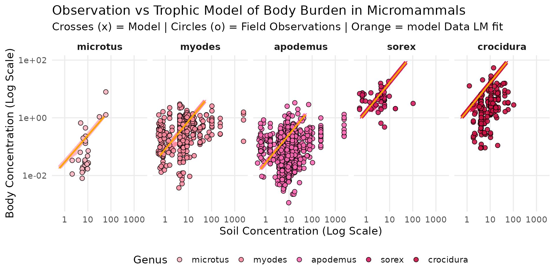
Mammals

micromammals_order <- c("microtus", "myodes", "apodemus", "sorex", "crocidura")
species_colors <- c(
  "beetle" = "#CD9B1D", "sorex" = "#D81B60", "microtus" = "#FFB6C1", 
  "myodes" = "#FF8DA1", "apodemus" = "#FF69B4", "turdus" = "#4169E1", 
  "columba" = "#87CEEB", "athene" = "#104E8B", "crocidura" = "#CC1144"
)

df_all_longer <- df_all |>
  dplyr::select(soil, myodes, microtus, apodemus, sorex, crocidura) |>
  tidyr::pivot_longer(
    cols = c("myodes", "microtus", "apodemus", "sorex", "crocidura"),
    names_to = "genus",
    values_to = "concentration"
  ) |>
  mutate(genus = factor(genus, levels = micromammals_order))


data("sf_micromammals")
sf_micromammals <- sf_micromammals |>
  mutate(genus = factor(tolower(genus), levels = micromammals_order))

ggplot() +
  theme_minimal(base_size = 14) +
  scale_x_log10() +
  scale_y_log10(limits = c(1e-3, NA)) +
  
  # On garde vos couleurs pour le trait (color) et le remplissage (fill)
  scale_color_manual(values = species_colors) +
  scale_fill_manual(values = species_colors) +
  
  # 1. MODÈLE EN ARRIÈRE-PLAN (Nuage de croix discrètes)
  geom_point(
    data = df_all_longer, 
    aes(x = 10^soil, y = concentration, color = genus), 
    shape = 4, 
    size = 1,      # Plus petit
    alpha = 0.2    # Forte transparence
  ) +
  # 3. OBSERVATIONS EN PREMIER PLAN (Cercles avec bordure noire)
  geom_point(
    data = sf_micromammals, 
    aes(x = cd_S, y = cd_WB_FW, fill = genus), 
    shape = 21,          
    color = "black",     
    size = 2.5,          
    stroke = 0.5,        
    alpha = 0.9
  ) +
    # 2. MODÈLE LINÉAIRE SUR LES Simulation(Ligne orange)
  geom_smooth(
    data = df_all_longer,                       # <- Changement ici !
    aes(x = 10^soil, y = concentration),                  # <- Changement ici !
    method = "lm",           
    color = "orange",        
    fill = "orange",         
    alpha = 0.4,             
    linewidth = 1            
  ) +
  
  facet_grid(~genus) +
  
  labs(
    title = "Observation vs Trophic Model of Body Burden in Micromammals",
    subtitle = "Crosses (x) = Model | Circles (o) = Field Observations | Orange = model Data LM fit",
    x = "Soil Concentration (Log Scale)",
    y = "Body Concentration (Log Scale)",
    color = "Genus",
    fill = "Genus"
  ) +
  theme(
    legend.position = "bottom",
    panel.grid.minor = element_blank(),
    strip.text = element_text(face = "bold", size = 12)
  )

Risk based on SSD

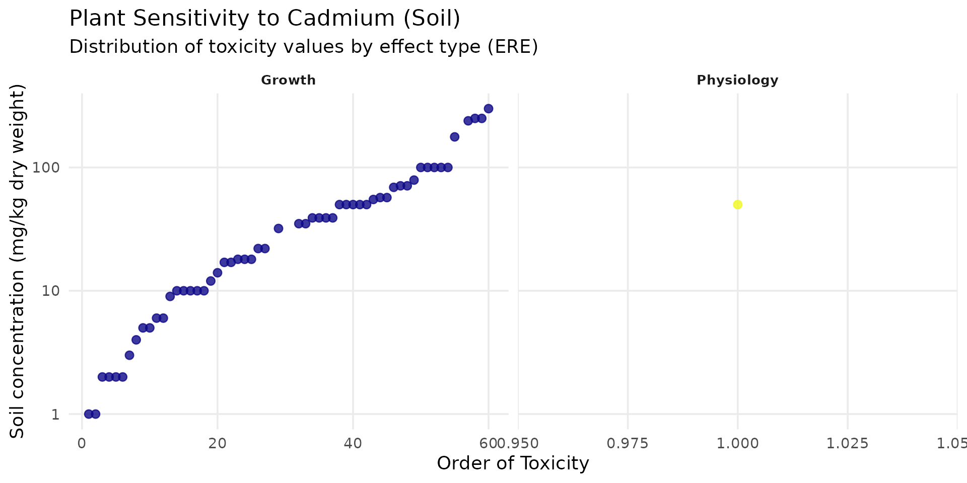
Define threshold

data("SSD_ecoSSL_all")

plants

ssd_cd_plant <- SSD_ecoSSL_all |>
  dplyr::filter(
    compound == "Cadmium",
    species_group == "Plant",
    !is.na(tox_value)
  )

# Create the plot
ggplot(data = ssd_cd_plant, aes(x = order_tox_value, y = tox_value, color = ERE_full)) +
  theme_minimal(base_size = 14) +
  # geom_hline(yintercept = 32, linetype = "dashed", color = "red", linewidth = 1) +
  geom_point(size = 2.5, alpha = 0.8) +
  facet_wrap(~ ERE_full, scales = "free_x") +
  scale_y_log10(labels = label_number()) +
  scale_color_viridis_d(option = "plasma", guide = "none") +
  labs(
    title = "Plant Sensitivity to Cadmium (Soil)",
    subtitle = "Distribution of toxicity values by effect type (ERE)",
    x = "Order of Toxicity",
    y = "Soil concentration (mg/kg dry weight)"
  ) +
  theme(
    panel.grid.minor = element_blank(),
    strip.text = element_text(face = "bold", size = 10)
  )

Invertebrates

ssd_cd_invert <- SSD_ecoSSL_all |>
  dplyr::filter(
    compound == "Cadmium",
    grepl("Invert", species_group), # Flexible filter for Invertebrates
    !is.na(tox_value)
  )

ggplot(data = ssd_cd_invert, aes(x = order_tox_value, y = tox_value, color = ERE_full)) +
  theme_minimal(base_size = 14) +
  geom_point(size = 2.5, alpha = 0.8) +
  facet_wrap(~ ERE_full, scales = "free_x", ncol=4) +
  scale_y_log10(labels = label_number()) +
  scale_color_viridis_d(option = "viridis", guide = "none") +
  labs(
    title = "Invertebrate Sensitivity to Cadmium (Soil)",
    subtitle = "Distribution of toxicity values by effect type (ERE)",
    x = "Order of Toxicity",
    y = "Soil concentration (mg/kg dry weight)"
  ) +
  theme(panel.grid.minor = element_blank(), strip.text = element_text(face = "bold"))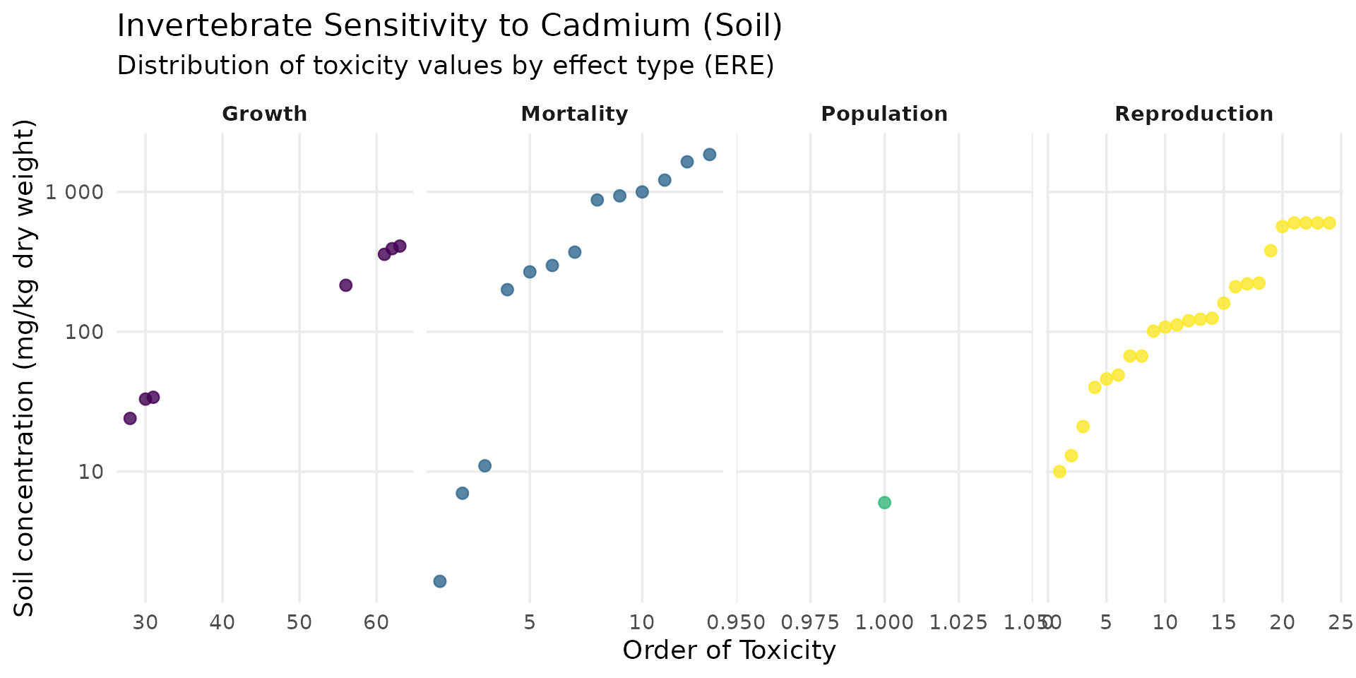

Mammals

ssd_cd_mammal <- SSD_ecoSSL_all |>
  dplyr::filter(
    compound == "Cadmium",
    grepl("Mammal", species_group),
    !is.na(tox_value)
  )

ggplot(data = ssd_cd_mammal, aes(x = order_tox_value, y = tox_value, color = ERE_full)) +
  theme_minimal(base_size = 14) +
  # geom_hline(yintercept = 0.77, linetype = "dashed", color = "red", linewidth = 1) +
  geom_point(size = 2.5, alpha = 0.8) +
  facet_wrap(~ ERE_full, scales = "free_x") +
  scale_y_log10(labels = label_number()) +
  scale_color_viridis_d(option = "magma", guide = "none") + 
  labs(
    title = "Mammal Sensitivity to Cadmium",
    subtitle = "Distribution of toxicity values (Daily Dose) by effect type",
    x = "Order of Toxicity",
    y = "Daily dose (mg/kg body weight / day)"
  ) +
  theme(panel.grid.minor = element_blank(), strip.text = element_text(face = "bold"))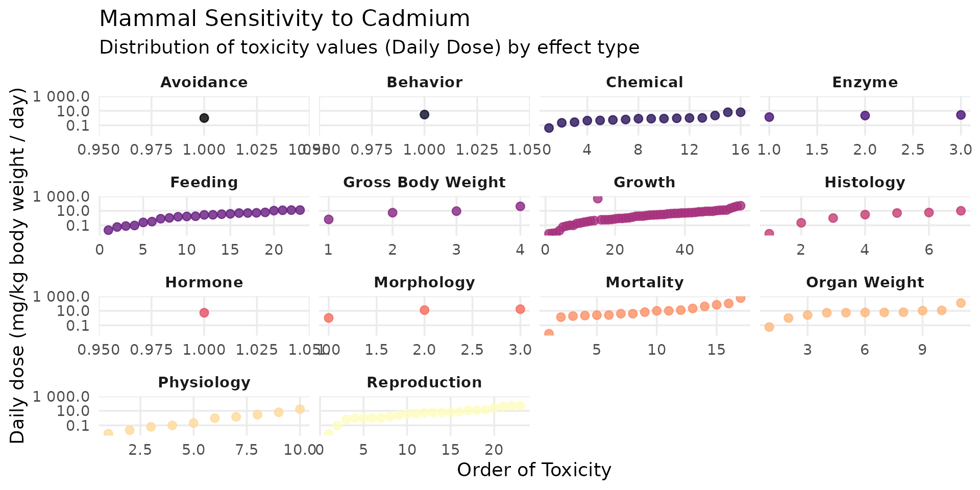

Birds

ssd_cd_avian <- SSD_ecoSSL_all |>
  dplyr::filter(
    compound == "Cadmium",
    grepl("Avian", species_group),
    !is.na(tox_value)
  )

ggplot(data = ssd_cd_avian, aes(x = order_tox_value, y = tox_value, color = ERE_full)) +
  theme_minimal(base_size = 14) +
  # geom_hline(yintercept = 1.47, linetype = "dashed", color = "red", linewidth = 1) +
  geom_point(size = 2.5, alpha = 0.8) +
  facet_wrap(~ ERE_full, scales = "free_x") +
  scale_y_log10(labels = label_number()) +
  scale_color_viridis_d(option = "cividis", guide = "none") +
  labs(
    title = "Bird Sensitivity (Avian) to Cadmium",
    subtitle = "Distribution of toxicity values (Daily Dose) by effect type",
    x = "Order of Toxicity",
    y = "Daily dose (mg/kg body weight / day)"
  ) +
  theme(panel.grid.minor = element_blank(), strip.text = element_text(face = "bold"))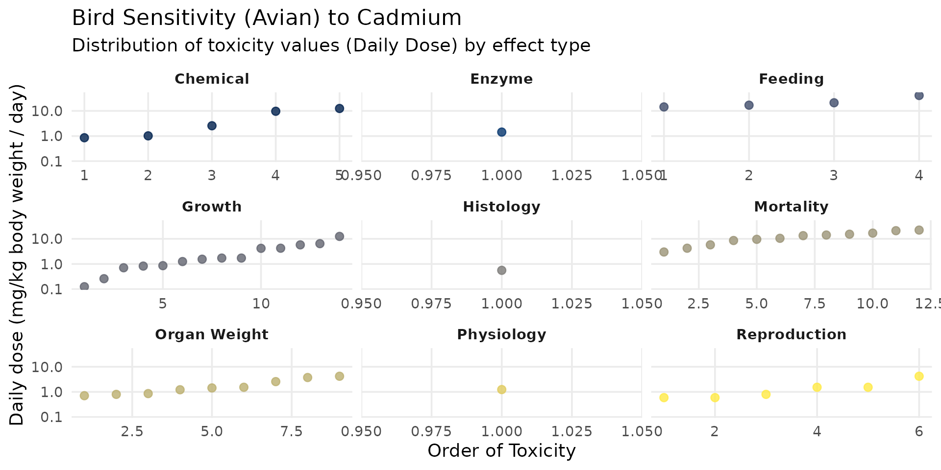

Risk Maps

Mortality

probs=0.5
plant_mortality = ssd_cd_plant[ssd_cd_plant$ERE_full=="Growth",]
plant_mortality_thrshld = quantile(plant_mortality$tox_value, probs=probs, na.rm=TRUE) |>
  as.numeric()

invert_mortality = ssd_cd_invert[ssd_cd_invert$ERE_full=="Mortality",]
invert_mortality_thrshld = quantile(invert_mortality$tox_value, probs=probs, na.rm=TRUE)|>
  as.numeric()

mammal_mortality = ssd_cd_mammal[ssd_cd_mammal$ERE_full=="Mortality",]
mammal_mortality_thrshld = quantile(mammal_mortality$tox_value, probs=probs, na.rm=TRUE)|>
  as.numeric()

bird_mortality = ssd_cd_avian[ssd_cd_avian$ERE_full=="Mortality",]
bird_mortality_thrshld = quantile(bird_mortality$tox_value, probs=probs, na.rm=TRUE)|>
  as.numeric()

# Reference thresholds for each component
# Reference thresholds for each component (Toutes les espèces incluses)
thresholds <- c(
  soil = 1,
  plant = plant_mortality_thrshld,
  earthworm = invert_mortality_thrshld,
  beetle = invert_mortality_thrshld,
  myodes = mammal_mortality_thrshld,
  microtus = mammal_mortality_thrshld,
  apodemus = mammal_mortality_thrshld,
  sorex = mammal_mortality_thrshld,
  crocidura = mammal_mortality_thrshld,
  columba = bird_mortality_thrshld,
  turdus = bird_mortality_thrshld,
  athene = bird_mortality_thrshld
)

# Align the vector's order with the raster layers' order (very important!)
ordered_thresholds <- thresholds[names(spcmdl_exposure)]
# Calculate the risk index: Concentration / Threshold
spcmdl_risk <-  spcmdl_diet_conc / ordered_thresholds
# Re-attach the trophic metadata since the division created a new object
spcmdl_risk <- spacemodel(spcmdl_risk, attr(spcmdl_diet_conc, "trophic_tbl"))

# Risk colors
breaks_risk <- c(-Inf, 0.1, 0.5, 1, 5, 10, Inf)
cols_risk <- c(
  "darkgreen",   # 0 - 0.1
  "green",       # 0.1 - 0.5
  "lightgreen",  # 0.5 - 1
  "yellow",      # 1 - 5
  "saddlebrown", # 5 - 10
  "#4A2C2A"      # > 10
)

names_keep <- names(spcmdl_risk)[names(spcmdl_risk) != "soil"]
spcmdl_risk_sub <- spcmdl_risk[[names_keep]]

terra::plot(spcmdl_risk_sub,
            breaks = breaks_risk,
            col = cols_risk)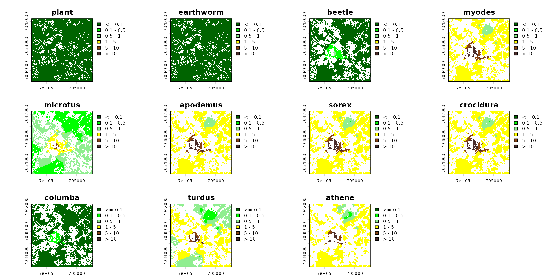

Reproduction

probs=0.5
plant_mortality = ssd_cd_plant[ssd_cd_plant$ERE_full=="Growth",]
plant_mortality_thrshld = quantile(plant_mortality$tox_value, probs=probs, na.rm=TRUE) |>
  as.numeric()

invert_mortality = ssd_cd_invert[ssd_cd_invert$ERE_full=="Reproduction",]
invert_mortality_thrshld = quantile(invert_mortality$tox_value, probs=probs, na.rm=TRUE)|>
  as.numeric()

mammal_mortality = ssd_cd_mammal[ssd_cd_mammal$ERE_full=="Reproduction",]
mammal_mortality_thrshld = quantile(mammal_mortality$tox_value, probs=probs, na.rm=TRUE)|>
  as.numeric()

bird_mortality = ssd_cd_avian[ssd_cd_avian$ERE_full=="Reproduction",]
bird_mortality_thrshld = quantile(bird_mortality$tox_value, probs=probs, na.rm=TRUE)|>
  as.numeric()

# Reference thresholds for each component
# Reference thresholds for each component (Toutes les espèces incluses)
thresholds <- c(
  soil = 1,
  plant = plant_mortality_thrshld,
  earthworm = invert_mortality_thrshld,
  beetle = invert_mortality_thrshld,
  myodes = mammal_mortality_thrshld,
  microtus = mammal_mortality_thrshld,
  apodemus = mammal_mortality_thrshld,
  sorex = mammal_mortality_thrshld,
  crocidura = mammal_mortality_thrshld,
  columba = bird_mortality_thrshld,
  turdus = bird_mortality_thrshld,
  athene = bird_mortality_thrshld
)

# Align the vector's order with the raster layers' order (very important!)
ordered_thresholds <- thresholds[names(spcmdl_diet_conc)]
# Calculate the risk index: Concentration / Threshold
spcmdl_risk <- spcmdl_diet_conc / ordered_thresholds
# Re-attach the trophic metadata since the division created a new object
spcmdl_risk <- spacemodel(spcmdl_risk, attr(spcmdl_diet_conc, "trophic_tbl"))

# Risk colors
breaks_risk <- c(-Inf, 0.1, 0.5, 1, 5, 10, Inf)
cols_risk <- c(
  "darkgreen",   # 0 - 0.1
  "green",       # 0.1 - 0.5
  "lightgreen",  # 0.5 - 1
  "yellow",      # 1 - 5
  "saddlebrown", # 5 - 10
  "#4A2C2A"      # > 10
)

names_keep <- names(spcmdl_risk)[names(spcmdl_risk) != "soil"]
spcmdl_risk_sub <- spcmdl_risk[[names_keep]]

terra::plot(spcmdl_risk_sub,
            breaks = breaks_risk,
            col = cols_risk)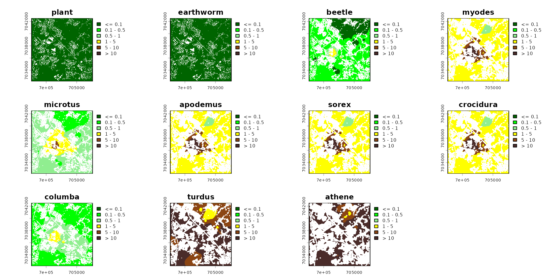

vs Eco-SSL

# Define the Eco-SSL thresholds (in mg/kg) for each group in a named vector
# 1. Valeurs de référence Eco-SSL (en mg/kg) pour chaque groupe écologique
ecossl_vals <- c(
  plant      = 32,
  invert     = 140,
  mamHerb    = 73,
  mamInsect  = 0.36,
  birdHerb   = 28,
  birdInsect = 0.77,
  birdCarn   = 630
)

# 2. Liste des kernels (NA car le calcul du seuil Eco-SSL est purement local / non dispersé)
ecossl_kernels <- list(
  soil = NA, plant = NA, earthworm = NA, beetle = NA,
  myodes = NA, microtus = NA, apodemus = NA, 
  sorex = NA, crocidura = NA, 
  columba = NA, turdus = NA, athene = NA
)

# 3. Construction des seuils Eco-SSL (Calcul du Quotient de Danger - HQ)
ecossl_threshold <- flux(spcmdl_berisp_flux, default = 1, normalize = FALSE) |>
  # Végétaux
  add_flux(from = "soil", to = "plant", value = ~ 10^x / ecossl_vals["plant"]) |>
  # Invertébrés
  add_flux(from = "soil", to = "earthworm", value = ~ 10^x / ecossl_vals["invert"]) |>
  add_flux(from = "soil", to = "beetle",    value = ~ 10^x / ecossl_vals["invert"]) |>
  # Mammifères - Herbivores / Omnivores
  add_flux(from = "soil", to = "myodes",   value = ~ 10^x / ecossl_vals["mamHerb"]) |>
  add_flux(from = "soil", to = "microtus", value = ~ 10^x / ecossl_vals["mamHerb"]) |>
  add_flux(from = "soil", to = "apodemus", value = ~ 10^x / ecossl_vals["mamHerb"]) |>
  # Mammifères - Insectivores
  add_flux(from = "soil", to = "sorex",     value = ~ 10^x / ecossl_vals["mamInsect"]) |>
  add_flux(from = "soil", to = "crocidura", value = ~ 10^x / ecossl_vals["mamInsect"]) |>
  # Oiseaux
  add_flux(from = "soil", to = "columba", value = ~ 10^x / ecossl_vals["birdHerb"]) |>
  add_flux(from = "soil", to = "turdus",  value = ~ 10^x / ecossl_vals["birdInsect"]) |>
  add_flux(from = "soil", to = "athene",  value = ~ 10^x / ecossl_vals["birdCarn"])

# Apply the transfer to compute the spatial risk layers
spcmdl_ecossl_risk <- transfer(
  spcmdl_berisp_flux,
  ecossl_kernels,
  ecossl_threshold,
  exposure_weighting="potential"
)

# Risk colors
breaks_risk <- c(-Inf, 0.1, 0.5, 1, 5, 10, Inf)
cols_risk <- c(
  "darkgreen",   # 0 - 0.1
  "green",       # 0.1 - 0.5
  "lightgreen",  # 0.5 - 1
  "yellow",      # 1 - 5
  "saddlebrown", # 5 - 10
  "#4A2C2A"      # > 10
)

names_keep <- names(spcmdl_ecossl_risk)[names(spcmdl_ecossl_risk) != "soil"]
spcmdl_ecossl_risk_sub <- spcmdl_ecossl_risk[[names_keep]]

terra::plot(spcmdl_ecossl_risk_sub,
            breaks = breaks_risk,
            col = cols_risk)

Trophic web

Plants and Beetles

Diet of mammals and birds: the EltonTraits 1.0 database

Small mammals: voles and shrew

Birds: little owl and black bird

Food Ingestion Rate per Body Weight

close species

FIR weighted

Habitat

Database of Habitat base on @oconnor2024habitat

Rasterize on a same grid frame

Create the spacemodel

Fluxes

Fluxes: Direct contamination (soil-target transfer for plant and earthworm)

Vegetation

Earthworm

spacemodel edit: implementing soil-vegetation and soil-earthworm fluxes

Fluxes: Trophic Contamination (Dietary Exposure)

A little bit of theory

Fluxes of Biomass FIRbw

spacemodel edit: implementing fluxes of biomass

Fluxes of Contaminants

Carabid

Mammals

Birds

spacemodel edit: implementing fluxes of contaminant

Movement of population (extended habitat) dispersion in landscape

Representation of kernels

Compute dispersal

Transfer of food and contaminant

Kernel of foraging

Body-Burden: compute impregnation

Exposure Extract exposure

Compared to data

Plants

Earthworm

Mammals

Risk based on SSD

Define threshold

plants

Invertebrates

Mammals

Birds

Risk Maps

Mortality

Reproduction

vs Eco-SSL

`spacemodel` edit: implementing soil-vegetation and soil-earthworm fluxes

`spacemodel` edit: implementing fluxes of biomass

`spacemodel` edit: implementing fluxes of contaminant