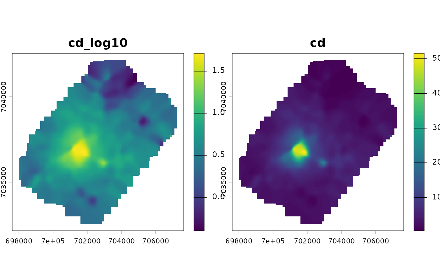
Gaussian kernel smoothing of soil concentrations

A simple, assumption-light alternative to kriging: the value of each cell is the weighted mean of the sampled values, the weights being a Gaussian function of the distance (Nadaraya-Watson estimator): $$\hat z(s) = \frac{\sum_i K(s - s_i) z_i}{\sum_i K(s - s_i)}$$

It re-uses [compute_kernel()] (the dispersal kernel of the package): the points are first rasterised (sum of values and number of points per cell), both rasters are convolved with the kernel using [terra::focal()], and the ratio gives the smoothed map.

Unlike kriging, the result does not honour the data and the smoothing strength (`radius`) must be chosen by the user, e.g. by cross-validation with [cv_soil()].

Usage

kernel_smooth_soil(
  points,
  value,
  radius,
  template = NULL,
  log10 = TRUE,
  res = 25,
  margin = 1000,
  size_std = 3,
  mask = NULL
)

Arguments

points

An `sf` object of POINT geometries in a projected CRS (metres).

value

Character. Name of the concentration column (e.g. `"cd"`).

radius

Numeric. Standard deviation (m) of the Gaussian kernel.

template

Optional `SpatRaster` defining the output grid. If `NULL`, a grid is built from the points with [soil_grid()] using `res` and `margin`. If `covariates` is given and `template` is `NULL`, the covariate grid is used.

log10

Logical. Krige `log10(value)` (default `TRUE`).

res, margin

Resolution and margin (m) of the grid built when `template` and `covariates` are `NULL`.

size_std

Numeric. Half-size of the kernel window, in number of `radius` (passed to [compute_kernel()]). Cells with no point within the window are `NA`.

mask

Optional `sf` polygon or `SpatVector`; cells outside are set to `NA`.

Value

A `SpatRaster` with the layer `<value>_log10` (or `<value>` if `log10 = FALSE`) and, if `log10 = TRUE`, the back-transformed layer `<value>`.

See also

[compute_kernel()], [krige_soil()], [cv_soil()]

Examples

data(soil_metaleurop)
r <- kernel_smooth_soil(soil_metaleurop, "cd", radius = 200, res = 50)
terra::plot(r)