Habitat and Connectivity

Introduction

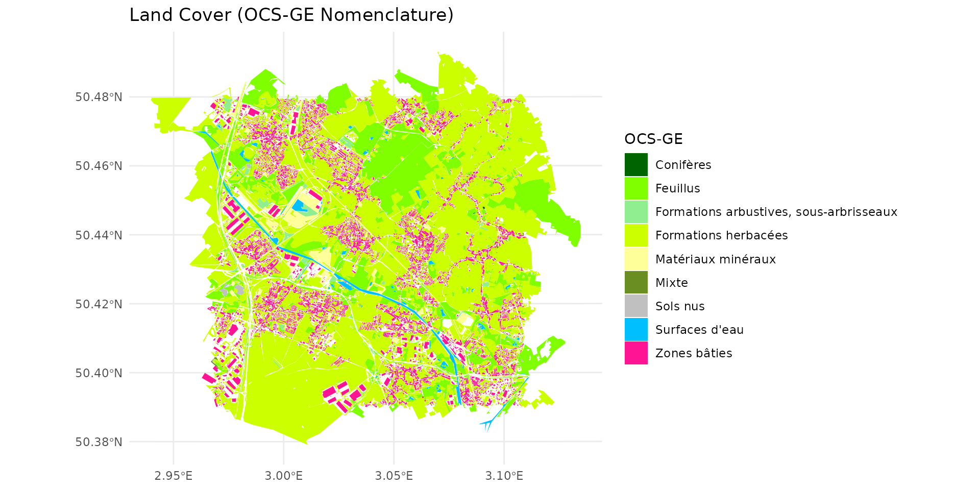
In this vignette, we explore the database linking OCS-GE (French GIS layer for Occupation du Sol à Grande Échelle) labels with species labels.

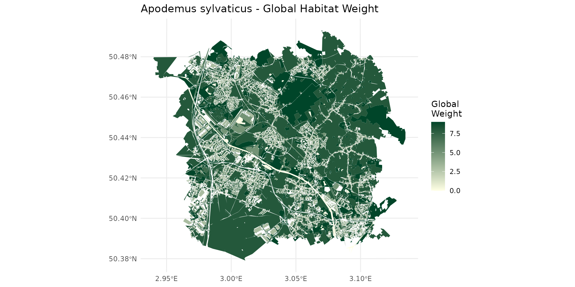
We will analyze how different land cover types act as habitats with varying qualities or resistances for different species, starting with the Wood mouse (Apodemus sylvaticus).

library(spacemodR)
library(dplyr)
library(ggplot2)
library(terra)
library(tidyterra)
library(sf)
library(leaflet)
library(patchwork)

Defining Habitat

Weighted species habitat with OCS-GE layer for Apodemus sylvaticus

First, we load the necessary datasets provided by spacemodR:

1. The species dictionary assigning weights to land cover codes.
2. The OCS-GE nomenclature reference (containing names and specific hex colors).
3. The spatial layer for OCS-GE (here, we use the ocsge_metaleurop dataset as our base map).

# Load the species dict and reference tables
data("ocsge_species_dict")
data("ref_ocsge")

# Load spatial data
data("ocsge_metaleurop") 
sf_ocsge <- ocsge_metaleurop

We filter our species dictionary for Apodemus sylvaticus and join it with the reference nomenclature to link the OCS-GE codes to their descriptive labels and predefined colors.

# Filter for Apodemus sylvaticus
dfhab_Apsy <- ocsge_species_dict[
  grepl("Apodemus_sylvaticus",ocsge_species_dict$nom_espece, ignore.case = TRUE), 
  ]

# Join ref_ocsge with the species dictionary. 
# ref_ocsge$code_cs_ (with spaces) matches ocsge_species_dict$code_cs
df_merged_Apsy <- ref_ocsge %>%
  dplyr::left_join(dfhab_Apsy, by = c("code_cs_" = "code_cs"))

# Join with the spatial sf object. Assuming sf_ocsge uses 'code_cs' (without spaces)
sf_Apsy <- sf_ocsge %>%
  dplyr::left_join(df_merged_Apsy, by = "code_cs")

Understanding Habitat Values

By examining the weight_global (wg), we can classify the landscape into different habitat qualities for the species:

• Non-habitat area (wg = 0):

df_merged_Apsy %>% 
  filter(weight_global == 0) %>%
  pull(nomenclature) %>%
  unique()
#> [1] "Surfaces d'eau"    "Névés et glaciers"

• Very Poor habitat (0 < wg <= 3):

df_merged_Apsy %>% 
  filter(weight_global > 0, weight_global <= 3) %>% 
  pull(nomenclature) %>% 
  unique()
#> [1] "Zones bâties"                    "Zones non bâties"               
#> [3] "Autres formations non ligneuses"

• Poor habitat (3 < wg <= 7):

df_merged_Apsy %>% 
  filter(weight_global > 7) %>% 
  pull(nomenclature) %>% 
  unique()
#> [1] "Feuillus"                               
#> [2] "Conifères"                              
#> [3] "Mixte"                                  
#> [4] "Formations arbustives, sous-arbrisseaux"
#> [5] "Formations herbacées"

• Good habitat (wg > 7):

df_merged_Apsy %>% 
  filter(weight_global > 7) %>% 
  pull(nomenclature) %>% 
  unique()
#> [1] "Feuillus"                               
#> [2] "Conifères"                              
#> [3] "Mixte"                                  
#> [4] "Formations arbustives, sous-arbrisseaux"
#> [5] "Formations herbacées"

Static Mapping

We will now visualize the spatial distribution of these metrics. We produce four maps focusing on Global Weight, Foraging Weight, Landscape Resistance, and finally the standard OCS-GE Land Cover.

Interactive Synthesis

To better explore the local variations and overlay different habitat parameters for Apodemus sylvaticus, we combine them into a single interactive leaflet map. You can toggle the layers in the top right corner.

Multi-species Interactive Synthesis

Different species interact with the landscape in radically different ways. Below, we create a function to automatically generate the interactive Leaflet synthesis for any given species, allowing us to rapidly compare their habitat preferences. ### Turdus merula (Blackbird)

turdus_hab <- join_ocsge_species(sf_ocsge, "Turdus_merula")
plot_species_habitat(turdus_hab)

Passer domesticus (House Sparrow)

passer_hab <- join_ocsge_species(sf_ocsge, "Passer_domesticus")
plot_species_habitat(passer_hab)

Small Mammals (Sorex, Crocidura, Microtus arvalis)

sorex_hab <- join_ocsge_species(sf_ocsge, "Sorex")
plot_species_habitat(sorex_hab)

crocidura_hab <- join_ocsge_species(sf_ocsge, "Crocidura")
plot_species_habitat(crocidura_hab)

microtus_hab <- join_ocsge_species(sf_ocsge, "Microtus_arvalis")
plot_species_habitat(microtus_hab)

Connectivity

From habitat to raster of source and resistance

1. first step is to collect habitat of the OCS-GE as we did previously

apsy_hab <- join_ocsge_species(sf_ocsge, "Apodemus_sylvaticus")
plot_species_habitat(apsy_hab)

2. then, we have to create an habitat object to benefit from spacemodR functionalities

apsy_habitat <- habitat(apsy_hab, habitat=TRUE, weight=apsy_hab$weight_global)
apsy_resistance <- habitat(apsy_hab, habitat=TRUE, weight=apsy_hab$resistance)

3. converting them in raster

ground_cd <- load_raster_extdata("ground_concentration_cd_compressed.tif")

rast_Apsy_habitat <- habitat_raster(ground_cd, apsy_habitat)

Note that for resistance, we have to use and exponential scale compare to the score in $[0-10]$ that with have in the data-set ocsge_species_dict to an exponential $[1-1000]$.

rast_Apsy_resistance_init <- habitat_raster(ground_cd, apsy_resistance)
exp_scl <- function(x) { 10^( (log10(1000) / 10) * x )}
rast_Apsy_resistance <- exp_scl(rast_Apsy_resistance_init)

par(mfrow = c(1, 2))
plot(rast_Apsy_resistance_init)
plot(rast_Apsy_resistance)

par(mfrow = c(1, 1))

terra::writeRaster(rast_Apsy_habitat, "julia_run/rast_Apsy_habitat.tif", overwrite = TRUE)
terra::writeRaster(rast_Apsy_resistance, "julia_run/rast_Apsy_resistance.tif", overwrite = TRUE)

Kernel

Omniscape

4. defining a radius

To define the radius, we have to know the real distance radius and then convert it into number of pixel. Let say, we have a dispersal radius of 500m for Apodemus sylvaticus, which is actually quite large for that species.

Here the map has pixels of 24m, so we use this large value for examples.

For pixel, the size is given by res(raster), here it is a meter system:

# get pixel size
terra::res(ground_cd)
#> [1] 24.93766 24.93976
# convert meter radius to pixel radius
m_radius = 500
px_radius = 500 / res(ground_cd)[1]
px_radius
#> [1] 20.05

docker run --rm \
  -v "$(pwd)/julia_run:/julia_run" \
  spacemodr Rscript /julia_run/run_dispersal.R \
  /julia_run/rast_Apsy_habitat.tif \
  /julia_run/rast_Apsy_resistance.tif \
  20.05 \
  omniscape_apsy_500m

docker run --rm \
  -v "$(pwd)/julia_run:/julia_run" \
  spacemodr Rscript /julia_run/run_dispersal.R \
  /julia_run/rast_Apsy_habitat.tif \
  /julia_run/rast_Apsy_resistance.tif \
  8.02 \
  omniscape_apsy_200m

p_src = ggplot() +
  theme_minimal() +
  geom_spatraster(data = rast_Apsy_habitat) +
  scale_fill_gradient(low = "#ffffe5", high = "#004529", na.value = "transparent", name = "Global\nWeight") +
  labs(title = "Source")

p_res = ggplot() +
  theme_minimal() +
  geom_spatraster(data = rast_Apsy_resistance) +
  scale_fill_gradient(
    low = "#fff5f0", high = "#67000d", transform="log10",
    na.value = "transparent", name = "Resistance")+
  labs(title = "Resistance")

max_r200m <- global(omniscape_apsy_200m, fun = "max", na.rm = TRUE)
norm_r200m <- omniscape_apsy_200m / as.numeric(max_r200m)
p_omn_200m = ggplot() +
  theme_minimal() +
  geom_spatraster(data = norm_r200m) +
  scale_fill_gradientn(
    colours = c("white", "#11dddd", "#dddd11", "red"),
    trans = "sqrt", 
    na.value = "transparent") +
  labs(title = "Omniscape Connectivity (r=200m)", fill = "Probability")

max_r500m <- global(omniscape_apsy_500m, fun = "max", na.rm = TRUE)
norm_r500m <- omniscape_apsy_500m / as.numeric(max_r500m)
p_omn_500m = ggplot() +
  theme_minimal() +
  geom_spatraster(data = norm_r500m) +
  scale_fill_gradientn(
    colours = c("white", "#11dddd", "#dddd11", "red"),
    trans = "sqrt", na.value = "transparent") +
  labs(title = "Omniscape Connectivity (r=500m)", fill = "Probability")

gridExtra::grid.arrange(p_src, p_res, p_omn_200m, p_omn_500m, ncol=2)